How Does Statistical Hypothesis Testing Work?

Statistically significant. p-value. Hypothesis.

These terms are not only commonly used in statistics but also have made their way into the vernacular. Making sense of most scientific publications, which can have practical, significant effects on public policy and your life, means understanding a core framework with which we derive much knowledge. That framework is called hypothesis testing, or more formally, Null Hypothesis Significance Testing (NHST).

When comparing two measurements, whether they be completion rates, ease scores, or even the effectiveness of different vaccines, a hypothesis test’s primary goal is to make a binary classification decision: is the difference statistically significant or not? Yes or no.

The yes or no output from a hypothesis test looks simple, indistinguishable from a guess or a coin flip. It’s the process of getting to yes or no that’s different in NHST.

While we certainly want to make the right decision, we can never be correct 100% of the time. There will always be mistakes; there will always be errors. It’s through the framework of hypothesis testing that we can control the frequency of errors over time.

Hypothesis testing can be a confusing concept, so we’ve broken it into steps with examples. In a follow-up article, we’ll discuss how things can go wrong in hypothesis testing and some criticisms of the framework.

Step 1: Define the Null Hypothesis

Statistical hypothesis testing starts with something called the Null Hypothesis. Null means none or no difference. A few ways to think of the Null Hypothesis are as the no-difference hypothesis or as the hypothesis that we want to nullify (disprove).

Mathematicians love using symbols, and that applies to hypothesis testing. The Null Hypothesis is represented as H₀. H stands for hypothesis, and the 0—that’s a zero in the subscript, not the letter O—reminds us it’s the hypothesis of 0 (no, null) difference.

We start with the Null Hypothesis because it’s easier to disprove something than to prove something. If we disprove the Null Hypothesis (reject the null), then we know there’s at least some relationship between the variables we’re measuring (e.g., different websites and ease scores).

Here are four examples of Null Hypotheses (H₀) from studies we’ll refer to throughout this article.

1. Rental Cars Ease: There’s no difference in System Usability Scale (SUS) scores between two rental car websites.
2. Flight Booking Friction: There’s no difference in perceived ease ratings (SEQ) when booking a flight on two airline websites.
3. CRM Ease: There’s no difference in System Usability Scale (SUS) scores between two Customer Relationship Management (CRM) apps.
4. Numbers and Emojis: There’s no difference in mean ratings on the UMUX-Lite when using numbers and face emojis as response options in its agreement scales.

Step 2: Collect Data and Compute the Difference

You need data to make decisions. Use methods such as surveys, experiments, and observations to collect data, and then calculate the differences observed. Data can be collected using either a between-subjects (different people in each condition) or within-subjects (same people in both) approach.

Building on the examples from Step 1,

1. Rental Cars Ease: 14 users attempted five tasks on two rental car websites. The average SUS scores were 80.4 (sd = 11) for rental website A and 63.5 (sd = 15) for rental website B. The observed difference was 16.9 points (the SUS can range from 0 to 100).
2. Flight Booking Friction: 10 users booked a flight on airline site A and 13 on airline site B. The average SEQ score for Airline A was 6.1 (sd = .83) and for Airline B, it was 5.1 (sd = 1.5). The observed difference was 1 point (the SEQ can range from 1 to 7).
3. CRM Ease: 11 users attempted tasks on Product A, and 12 users attempted the same tasks on Product B. Product A had a mean SUS score of 51.6 (sd = 4.07) and Product B had a mean SUS score of 49.6 (sd = 4.63). The observed difference was 2 points.
4. Numbers and Emojis: 240 respondents used two versions of the UMUX-Lite, one with a standard numeric format and the other using face emojis in place of numbers. The mean UMUX-Lite rating with the numeric format was 85.9 (sd = 17.5), and for the face emojis version, the score was 85.4 (sd = 17.1). That’s a difference of .5 points on a 0-100–point scale.

Table 1 summarizes the four examples (metrics and observed differences).

				Sample 1			Sample 2
No.	Example	Experimental Design	Metric	Mean	SD	N	Mean	SD	N	Difference
1	Rental Car	Within-subjects	SUS	80.4	11	14	63.5	15	14	16.9
2	Flight Friction	Between-subjects	SEQ	6.1	0.83	10	5.1	1.5	13	1
3	CRM Ease	Between-subjects	SUS	51.6	4.07	11	49.6	4.63	12	2
4	Numbers and Emojis	Within-subjects	UMUX-Lite	85.9	17.5	240	85.4	17.4	240	0.5

Table 1: Descriptive statistics (mean, standard deviation, and sample size) and differences for the four examples.

Step 3: Compute the p-value

With these differences computed, we want to know how likely it is they could have happened by chance. To do so, we use the probability value—the p-value.

Books are written on the p-value. Statisticians love to argue over its technical definition (similar to how UX practitioners and researchers argue over the definition of UX). In short, p-value is the probability of getting the differences we found in Step 2 if there really are no differences.

This often gets simplified as the probability that the difference is due to chance. Technically, that’s not quite correct, but it’s conceptually close enough for practical purposes (just watch whom you say it to).

We explain how to compute the p-value by hand for many common statistical tests in Chapter 5 of Quantifying the User Experience. But you’ll usually use statistical software such as SPSS or R to compute the p-value. (p-values are computed automatically in our MUIQ platform, as shown in Figure 1.)

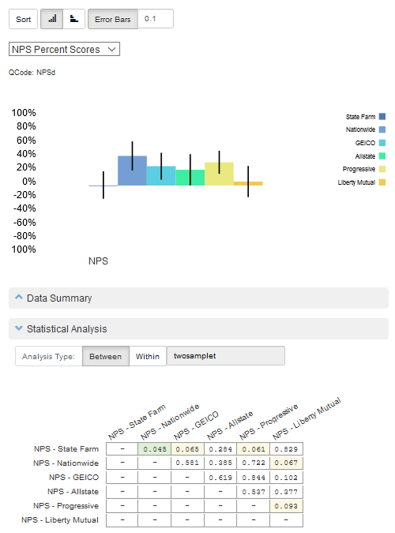
Figure 1: MUIQ output that compares the Net Promoter Scores for six auto insurance websites; the statistical analysis table shows the p-values for all the possible comparisons, with green highlights for p < .05 and yellow highlights for .05 < p < .10.

1. Rental Cars Ease: Used a paired t-test to assess the difference of 16.9 points (t(13) = 3.48; p = .004).
2. Flight Booking Friction: The observed SEQ difference was 1 point, assessed with an independent groups t-test (t(20) = 2.1; p = .0499).
3. CRM Ease: An independent groups t-test on the difference of 2 points found t(20) = 1.1; p = .28.
4. Numbers and Emojis: A dependent-groups t-test on the difference of .5 points found t(239 = .88; p = .38.

The lower the p-value, the less credible the Null Hypothesis is (or as is often interpreted, it’s less likely the difference is due to chance). But how low is low enough?

Step 4: Compare p-value to Alpha to Determine Statistical Significance

The p-value is compared to a criterion called the alpha error (α). If p is less than the criterion, then you can declare statistical significance (sort of like Michael Scott from The Office—Figure 2). When p is below alpha, we reject the Null Hypothesis.

Figure 2: Declaring statistical significance with a meme.

The most common criterion is .05 (the basis for saying that p < .05 indicates statistical significance). It doesn’t always have to be .05, but that’s what most scientific journals have adopted. We’ll cover how that threshold became the default in another article.

When something is statistically significant, it doesn’t mean it’s different. It just means we wouldn’t expect to see a difference that large if there really was no difference. Or if the null hypothesis is true, we would not expect to see the difference very often.

Let’s compare the p-values to the typical alpha criterion of .05 for our sample data to see whether there are any statistically significant differences:

1. Rental Cars Ease: The 16.9 difference has a p-value of .004. We’d expect a difference this large or larger only about 4/1000 times if there is no difference. p is less than .05. Statistically significant.
2. Flight Booking Friction: The observed difference of 1 point generated a p-value of .0499. We’d expect to see this difference just under 5% of the time if there was no difference. p is less than .05. Statistically significant.
3. CRM Ease: The 2-point difference generated a p-value of .28. A difference this large or larger could happen 28% of the time if there is no difference. p is greater than .05. NOT significant.
4. Numbers and Emojis: The .5-point UMUX-Lite difference generated a p-value of .38. If there is no difference, you’d expect to see a p-value this large 38% of the time. p is greater than .05. NOT significant.

Table 2 shows the four examples, the observed differences, resulting p-values, and conclusions.

No.	Example	Difference	p	Alpha	Statistically Significant
1	Rental Car	16.9	0.004	0.05	Yes
2	Flight Friction	1	0.0499	0.05	Yes
3	CRM Ease	2	0.28	0.05	No
4	Numbers and Emojis	0.5	0.38	0.05	No

Table 2: Observed differences, resulting p-values, and conclusions for the four examples.

The Path to Statistical Significance

We have visualized these steps in a flowchart (Figure 3).

When the difference is statistically significant (p < alpha) you reject the Null hypothesis (H₀). If p > alpha you can say something is not statistically significant, so you do not reject the Null Hypothesis. But, more importantly, you also do not accept it. There might be no difference, but it’s also possible that there is a real difference. The difference might be too small to detect with the given sample size and variability of measurement, making the outcome ambiguous. Strictly speaking, you fail to reject the Null Hypothesis (H₀). The language is subtle: the important point is you never accept the Null Hypothesis as true; you can only reject it (p < alpha) or fail to reject it (p > alpha).

In a future article, we’ll discuss other aspects of hypothesis testing, including the specification of an alternative hypothesis and how that expands the framework of NHST to define the two ways decisions can be right and the two ways they can be wrong.

 

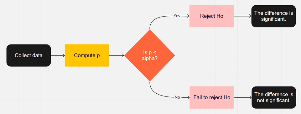
Figure 3: High-level flowchart of statistical hypothesis testing.

Summary

When making decisions in research, business, or even medicine, we can’t be correct 100% of the time. There will always be mistakes; there will always be errors. Through the framework of hypothesis testing, we can measure and reduce the frequency of errors over time. To use hypothesis testing when making comparisons, follow these four steps:

1. Define the Null Hypothesis. If we can rule out no difference, then we can conclude there’s at least some difference between the variables.
2. Collect data and compute the difference. Just because you observe a difference doesn’t mean it’s greater than what you’d see from sampling error or random fluctuation.
3. Compute the p-value. The probability value (p-value) is the probability of observing that difference or a larger one if there really is no difference.
4. Compare the p-value to alpha to determine statistical significance. If the p-value is less than the alpha criterion (typically .05), we conclude the difference is statistically significant. Otherwise, we withhold final judgment and can only say we failed to reject the Null Hypothesis.