 Know your data.
When measuring the customer experience, one of the first things you need to understand is how to identify and categorize the data you come across.
It’s one of the first things covered in our UX Boot Camp and it’s something I cover in Chapter 2 of Customer Analytics for Dummies.
Early consideration of your data types enables you to do the following:
- Summarize the data properly and compute the correct confidence interval.
- Evaluate the strengths and weaknesses (limitations) of each data type.
- Select the appropriate statistical test when making comparisons.
- Determine the right method for computing the study sample size.
Data classification can be confusing because it seems like there is an endless list of labels and categories you’ve probably encountered. While you can classify data in a number of ways, two of the most common and helpful ways are shown in the diagram below.
First, you can classify data as either qualitative or quantitative. Then, you can further classify quantitative data down into further subtypes.
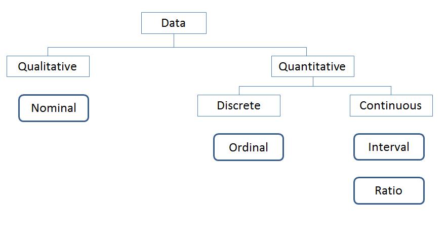
Qualitative and Quantitative Data Types
Qualitative data includes nonnumeric actions, descriptions, attributes, and qualities of user behavior and artifacts: software, websites, and mobile devices. Quantitative data includes anything described numerically: revenue, task time, rating scales—anything that can be counted.
We can break down quantitative data into two groups: discrete and continuous.
Discrete: Countable items that can’t be logically subdivided, such as the number of errors (you can’t have half an error) or the number of calls to tech support are considered discrete. Discrete data that has only two values is a called discrete-binary data. Task-completion rates (success or failure) or conversion rates (purchase or didn’t purchase) are examples of discrete-binary data.
Continuous: Data points that can fall anywhere on a continuum are called continuous. Here are some examples of continuous data: the time it takes to find a product on a website (say, 31.627543 seconds); or the dimensions of a cell phone (length and width), the distance to the nearest retail store, or the time it takes customers to find information on a website.
Levels of Data
Another way customer data gets divided is by the four levels of measurement: nominal, ordinal, interval and ratio. They’re levels because they start with data that’s generally more limiting in the type of claims you can make to the least limiting.
Nominal: Nominal means “in name only,” so anything with a name belongs in this category. Nominal data is qualitative data. The name of your company, the type of car you drive, or the name of a product are all examples of nominal data. Even though nominal data is qualitative, it can still be counted.
Ordinal: Ordered data. The ranking of customers by oldest to newest, the order of callers in a queue for a call center, the order of runners finishing a race, or more often, an ordinal choice on a rating scale (“On a scale of 1 to 5, how do you satisfied are you…?”).
Ordinal data cannot tell you with certainty whether the intervals between values are equal. In measuring customers’ attitudes toward their experience with products and services, you have to rely heavily on questionnaire data that uses rating scales. For example, on an 11-point rating scale, the difference between a 9 and a 10 is not necessarily the same as the difference between a 6 and a 7. Most rating scales you’ll encounter (including ones made up in surveys) are ordinal.
So just because customers’ average rating on one product is a 4 and the rating on another product is a 2 doesn’t mean customers are twice as satisfied. The first rating is twice as high as the second, but unless the scale is calibrated such that the numbers correspond to customer behavior, making such claims is risky. It’s best to simply say the rating was twice as high.
Interval: Data with equal interpreted distance between values. The most common example is temperature in degrees Fahrenheit. The one-degree difference between 29 degrees and 30 degrees is identical in magnitude to the one-degree difference between 78 degrees and 79 degrees (but it’s inaccurate to say something is twice as hot on this scale).
In practice, you’ll rarely run into a true interval scale. The SMEQ is one of the few I’ve used. Using Item Response Theory (IRT), however, can convert ordinal response scales into interval data based on how participants respond. I’ll have more to say about IRT in future posts.
Ratio: Interval data with a meaningful zero point. Time taken to find a product on a website is ratio data, because 0 time is meaningful. Degrees Kelvin has a 0 point (absolute zero). Each one-step interval in each scale has the same degree of magnitude as every other step. Whenever you can establish that data is ratio, you can make reasonable deductions, such as “customers are twice as satisfied using a new product version compared to an old version.” Notice the ratio you get when you divide two customer satisfaction numbers–hence, ratio data. There’s been some work, called Usability Magnitude Estimation, to apply ratio scaling to perceptions of usability. We found limited success[pdf] with these, as participants found them difficult to use; and we got similar results using a simple ordinal scale which became the basis of the SEQ. In practice, task-time is one of the most common ratio level metrics you’ll encounter.
Some Brief History on the Levels of Measurement
Where did the levels of measurement come from, and why should you care? In the 1940s, when behavioral science was in its infancy, there was much concern about legitimizing behavioral science. Along with psychology and other social sciences, behavioral science is considered a soft science, in contrast to the hard sciences: chemistry and physics. It was hoped that applying thinking from hard sciences would improve the legitimacy of the soft sciences and thereby bolster acceptance of the claims made. One approach (proposed by S.S. Stevens in 1946) was to map types of scaling to more natural laws—something akin to the physical laws of gravity and motion. Stevens said that you should take averages on, at the least, interval and ratio data. Nominal and ordinal data should be counted and described only in frequency tables—no means and no standard deviations.
One of the more famous articles showing the fallacy of such rigid thinking was by an eminent statistician named Frederic Lord, who in his article “On the Statistical Treatment of Football Numbers” showed how the means of nominal data can be meaningful too! Lord went on to run ETS, the company behind the SAT.
In practice, it’s generally OK to take means and apply statistical tests to ordinal data (everyone does it because you get such useful results!), but be careful about making ratio claims such as “twice as satisfied.”
Conclusion
When working with your data, keep the following in mind:
- Determine whether you have qualitative or quantitative data: Qualitative data limits the type of statistical analysis you can perform, but at the very least you can still count, and summarize the counts of, observations, names, and other non-numeric attributes.
- Identify quantitative data as discrete or continuous: Discrete data is countable (e.g. number of errors) and is often binary (having only two options) such as purchased/didn’t purchase. Continuous data provides more fidelity and therefore requires a smaller sample size to detect differences. Where possible, look to collect more continuous measures; you can always decompose a continuous measure down to a discrete or binary measure (for example, customers took more than 2 minutes or less than 2 minutes).
- Rating-scale data, while technically discrete, can often be treated continuously as long as you’re careful about the claims you make (e.g. don’t say customers are twice as satisfied!).
- Continuous data that is interval or ratio has equal distances between values. Ratio data has a 0 point which means statements like “twice as long” can be made. It’s unusual to see ratio scales in use in the behavioral sciences.
In practice, we’ve found that once you identify your data as quantitative, you need to know mainly whether you’re working with continuous or discrete binary data to determine the best statistical test and method for finding the sample size. So while it’s good to understand how data can get classified, especially when having discussions with other numerically minded stakeholders, don’t get too caught up in the measurement classifications.
Make sure that more effort is spent on doing something about the data you collect than on just classifying it.


