 Excel is a powerful program. It’s like an onion, peeling back layers to reveal increasingly specialized functions.
The minute you think you’ve mastered it, you discover a new set of functions.
It can take years to learn it and unfortunately there’s not usually a class on learning Excel in university. Students have to pick things up on their own.
But after you get beyond the basic idea of the spreadsheet and understand how simple formulas like =COUNT(), =AVERAGE(), and =SUM() work, you should master the following 5 functions and techniques that make data analysis more efficient and powerful.
This is the first of two articles on using Excel for data analysis.
1. IF (Conditional)
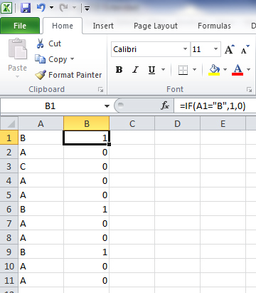
Conditionals are essential components of every programming language and it’s the same for Excel. If you want to count how many people selected “B” as a response, use the IF function.
The formula is =IF (A1=”B”, 1,0). This tells you that if the value in cell A1 is B, then display a 1; otherwise display a 0. You can then copy the formula for each subsequent row and average the columns =AVERAGE(B:B) to find the proportion that selected a B. See the following figure and download the spreadsheet with the examples.
2. COUNTIF
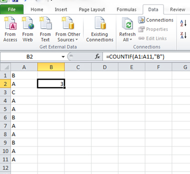
You do a lot of counting in Excel when doing an analysis. Counting has a conditional function, too. Building on the last IF statement, if you want to count how many Bs were identified, use the formula = COUNTIF(A1:A11,”B”). Select the range (cells A1 to A11) and the criteria (in this case the criteria is a B) as shown in the figure below.
3. Transpose
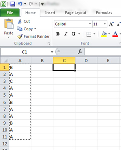
Researchers should be prepared for data to come in just about any format. The first thing you’ll need to do is organize your data for efficient analysis, and this often means changing the orientation of data. If you want data to go from horizontal to vertical (or vice versa), you want to transpose. Follow these steps to transpose values.
1. Copy the values you want to transpose.
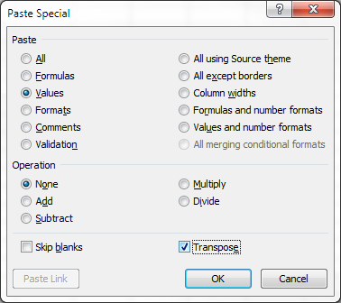
2. Right-click the selected cells and select Paste Special.
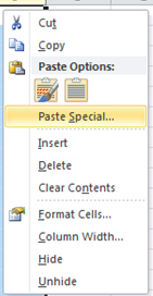
3. Select the Transpose check box at the bottom. Click OK. You’ll often want to paste just the values (and not any formulas that may lose their reference cells).
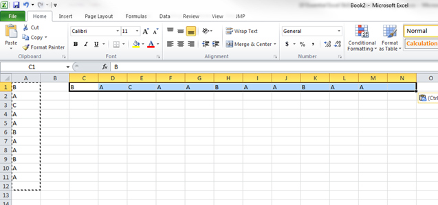
Your values are then transposed from vertical to horizontal as shown in the figure below.
4. The Fill Handle
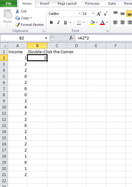
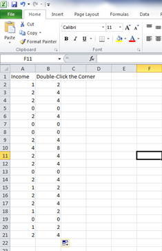
Double-clicking the right corner of a cell with a formula in Excel will cascade the formula down like magic. It’s called the fill handle. For example, if you want to apply a simple formula, such as one to double values, instead of holding and dragging your mouse down the column, double-click the corner of the cell. This trick alone will save most people plenty of frustration!
 |
 |
5. Absolute Reference ($)
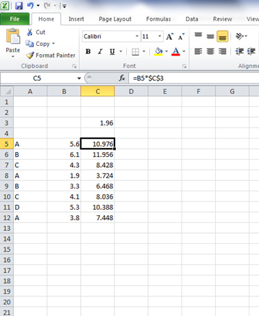
When you want to drag a formula down a column but want to keep referencing the same cell, you want to use an absolute reference. Excel uses the dollar sign $ for this function. For example, in the figure below I wanted to multiply each value by 1.96 (the value in cell C3).
I created the formula once and then added the dollar signs before and after the reference (C3 becomes $C$3). You can also press F4 on Windows and Command t on the Mac. Then I double-clicked the corner to use the fill handle and applied the formula to all the cells.
In part 2 of this article I’ll cover more advanced techniques that mimic database functions, including Pivot Tables and the Vlookup.

