A New Statistical Approach for Predicting Usability Problems

In an earlier article, we described the most common methods for modeling the total number of unique usability problems uncovered in a usability test: the average problem occurrence (p), adjusted problem occurrence (adj-p), beta-binomial, and specific problem probabilities.

While these methods provide reasonably accurate predictions of the total number of unique problems, there is still room for improving their accuracy (which is true of all models).

A relatively new approach for modeling problem discovery was suggested by Bernard Rummel in a personal communication. It’s based on a pattern he noticed: the total number of unique problems tends to have a linear relationship with the cube root of the sample size.

One of the challenging aspects of modeling the total number of problems left to find is that if you keep adding users, you’ll keep finding new problems. In this respect, interfaces aren’t static ponds with a fixed number of fish available to catch, but rather adding more fishermen (users) leads to the capture of more fish.

In short, the more users tested, the more unique problems are found, but with a diminishing return. Rummel proposed modeling the diminishing return with a regression equation that uses the cube root of the sample size on the first few participants. This approach is similar in this respect to the p and adjusted-p methods, which use the first few respondents to help build a model of future unique problem discovery.

For example, Figure 1 shows the total number of problems found for each of the first five participants in a usability study. (For the raw data, see Table 2 in the appendix.)

In the top graph, the dashed line shows a curved “cubic” relationship between the number of users and the cumulative number of unique problems. The bottom graph illustrates how modeling unique problem discovery with the cube root of the sample size works well with linear regression.

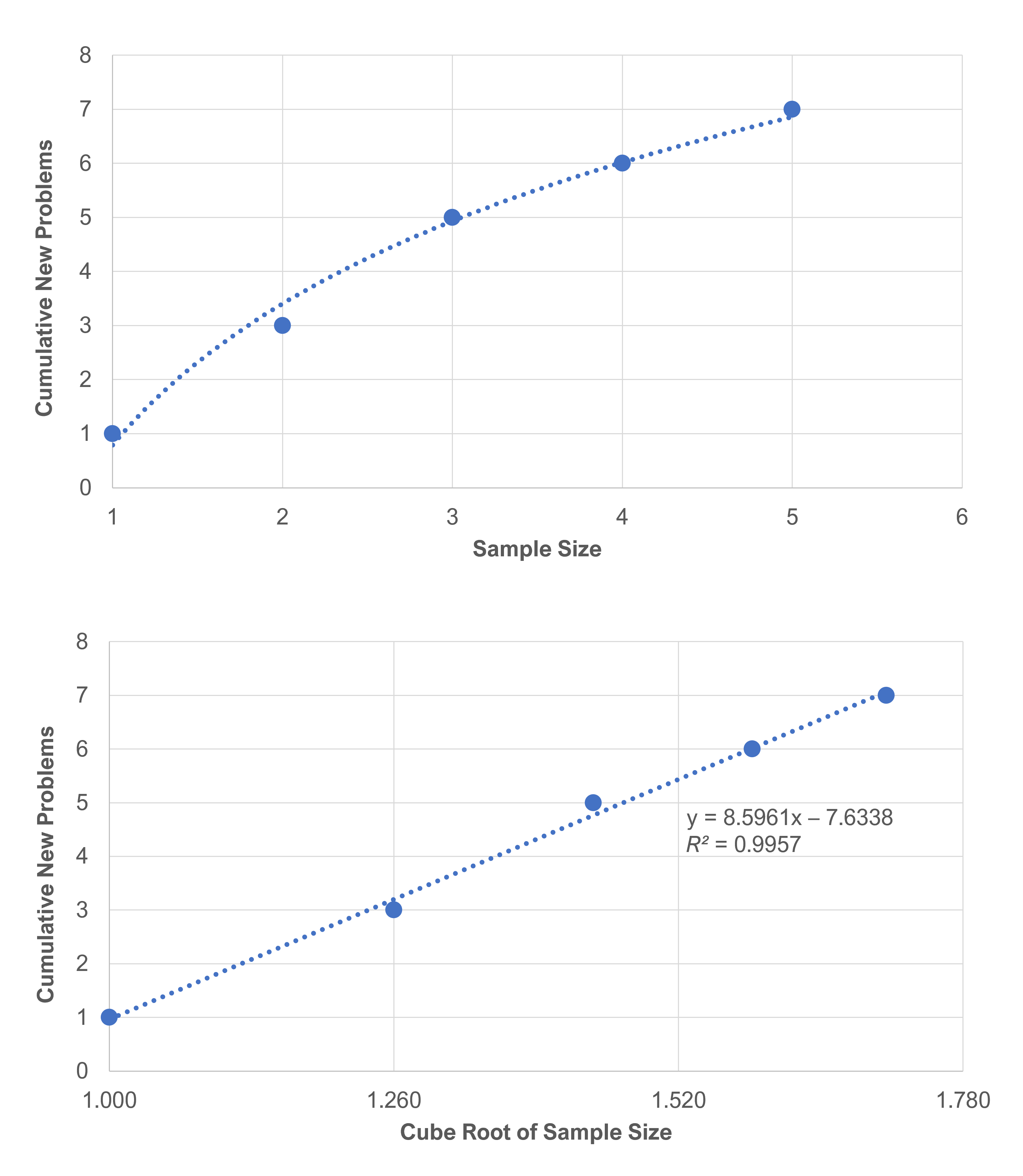
Both graphs show that the number of total usability problems will always increase with the addition of new users. If there was a finite number of problems the line would eventually flatten out on the top graph.

To find the cube root of a number, you raise it to the power of 1/3. For example, the cube root of 2 is 2^1/3 = 1.260, and the cube root of 8 is 2 (8^1/3 = 2, 2³ = 8). We don’t encounter the cube root very often, but think of it like the square root, which we do see in many statistics equations. You can find the square root of a number by raising it to the power of 1/2. Both the square and cube root are types of nonlinear transformations.

As shown in Figure 1, after converting sample sizes into their cube roots, we can then use a line (linear equation) to model their relationship with cumulative unique problem discovery.

With a linear equation, the slope and intercept are used to predict the expected number of unique problems to be discovered with a larger sample size. (For more on regression analysis see Chapter 10 in Quantifying the User Experience.)

The appealing thing about this approach is that it’s relatively simple to compute and understand, and it tends to match what we’ve seen in practice: a small number of yet unseen problems continue to appear even after testing many users. As we have done with the other models for predicting problems, we wanted to test its predictive abilities using real-world problem sets.

The Problem Sets

To assess the predictive ability of this approach, we used 15 usability problem datasets that all had relatively large sample sizes (n = 18 to n = 50). Some of the problem sets included problems aggregated across multiple tasks and some included only one task. The studies focused on both business web applications and consumer websites. The studies include a mix of in-person moderated studies and unmoderated studies where an observer coded problems from video recordings. Eight of the datasets come from U.S. health insurance websites and two from U.S. rental car websites.

Results

Table 1 shows the total number of unique problems uncovered in each of the studies, what was predicted by the regression equation after five participants, and the difference between the total predicted and the total discovered.

Generally Accurate but Highly Variable

Across the 15 datasets, the average predicted difference was off by only 2.1 problems (on average, a difference of 2%). That looks pretty impressive, but that small value doesn’t reveal a lot of variability with some datasets over and under predicting by a large amount. Using the absolute value of the difference, the number of problems predicted differs from the actual number by 6.2 (on average, a difference of 29.2%).

Another way to quantify the effect of variability is to compute confidence intervals for these estimates. With 95% confidence, intervals ranged from −21% to 25% for raw differences and from 14% to 44% for absolute differences.

Study	Sample Size	Total Problems Uncovered	Predicted Problems at 5	Raw Diff (Actual-Predicted)	Raw % Diff	ABS Diff	ABS % Diff
Health Insurance Website B T1	37	12	11.9	0.1	1%	0.1	1%
B2B App	18	41	39.6	1.4	3%	1.4	3%
Enterprise Website	45	33	34.6	−1.6	−5%	1.6	5%
IT App 1	30	131	122	9	7%	9	7%
Health Insurance Website C T2	44	23	21	2	9%	2	9%
Health Insurance Website B T2	37	10	8.5	1.5	15%	1.5	15%
IT App 2	30	101	84.4	16.6	16%	16.6	16%
Health Insurance Website A T1	39	10	8.2	1.8	18%	1.8	18%
Health Insurance Website A T4	37	17	13.4	3.6	21%	3.6	21%
Real Estate Website	20	11	7.5	3.5	32%	3.5	32%
Health Insurance Website A T2	39	10	6.2	3.8	38%	3.8	38%
Budget Website	38	24	36.7	−12.7	−53%	12.7	53%
Health Insurance Website A T3	37	10	15.7	−5.7	−57%	5.7	57%
Credit Card Mobile App	50	25	6.5	18.5	74%	18.5	74%
Health Insurance Website C T1	44	12	22.7	−10.7	−89%	10.7	89%
95% CI upper limit				6.7	25%	9.4	44%
Average				2.1	2%	6.2	29%
95% CI lower limit					−21%	2.9	14%

Table 1: Difference between predicted and actual observed unique usability problems using a regression equation with the cube root of the sample size as the only independent variable.

Why Such High Variability?

To get insight into the source of the high variability, we examined the individual datasets. For example, analysis of the first five datasets named in Table 1 shows the average absolute difference between predicted and observed problems was within 10%. For one of the health insurance websites (the first row in the table), the total unique number of problems predicted was very accurate even after 37 users. An IT app that had 131 problems from 6 tasks was predicted to have 122 problems, off by 9. In contrast, another health insurance website with only 1 task from 44 participants had 12 unique problems but the prediction was 22.7 problems, off by a substantial 89%.

For such a relatively simple method, the predictive accuracy for absolute differences was very good in five studies (<10% difference), modest in five studies (15% to 32%), and relatively poor in five (38% to 89%). The overall predictive accuracy for raw differences was excellent (2% difference), but the confidence interval around that estimate ranged from −21% to 25%.

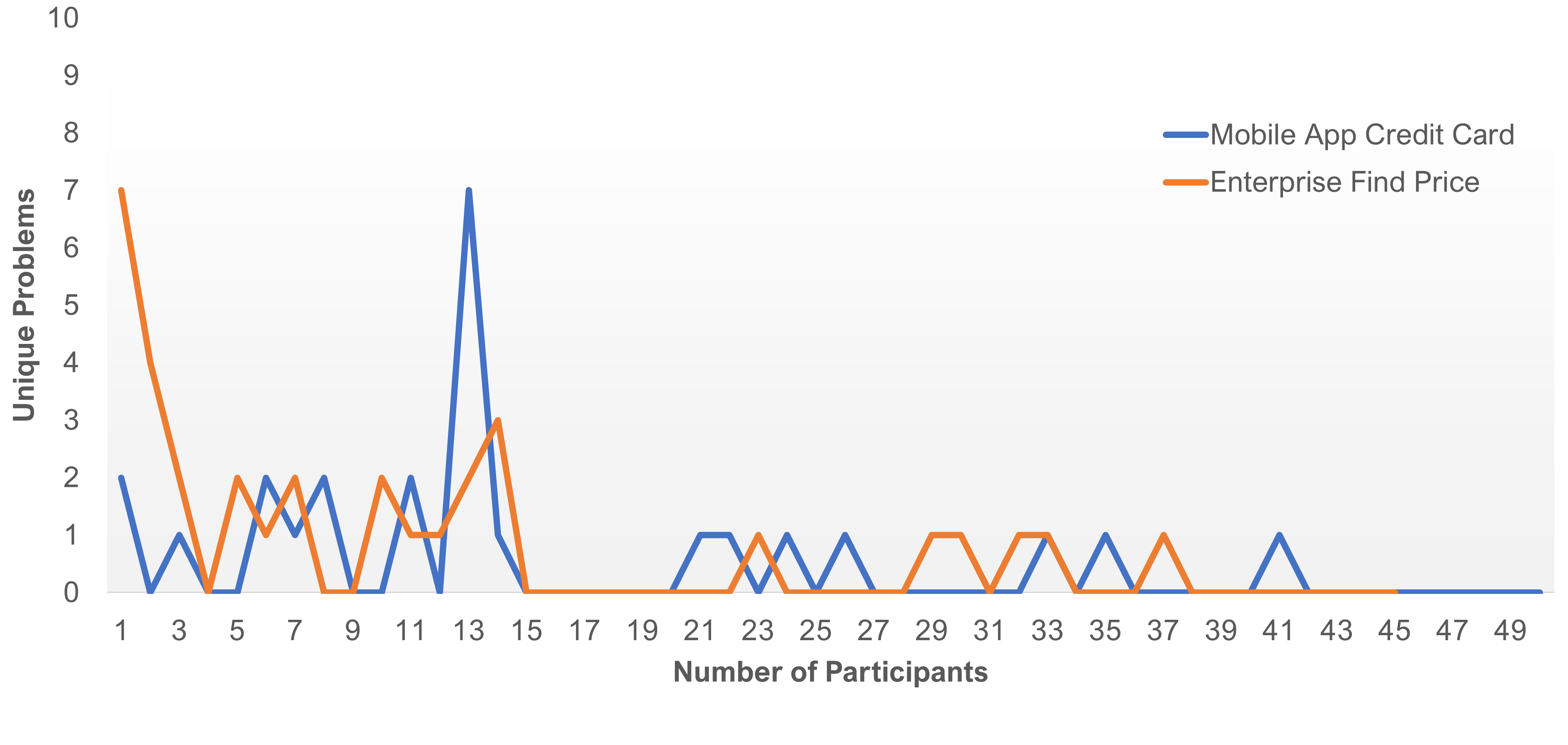
We looked more in-depth at the five datasets that had the highest error between prediction and actual unique problems observed. For regression analysis to work, we need to have a good idea about the frequency of new problems in the first five users. And across many of the datasets, we do see that most of the new problems happen relatively early (as we’d expect). However, in some datasets, for example, in the Credit Card Mobile study, the 13^th participant encountered seven new problems. You can see in Figure 2 how that looks compared to the more typical pattern of discovery in the Enterprise Rent-a-Car study.

While it’s likely there will always be a possibility of unexpected problem discovery, we believe there are at least three additional reasons that may contribute to an unexpectedly high number of new problems after the first few participants.

1. Design teams change focus: Usability testing is of course meant to identify and fix problems, not produce pristine datasets for us to analyze. As such, it’s not uncommon for design teams to change the focus of a study midway through to make the most of participant time and budgets. This often involves adjusting tasks or having a research moderator probe different areas, which consequently may uncover novel usability issues.
2. New user types encountered: We have seen cases where a participant who meets the screening criteria exhibits behavior different from prior participants. Participants may have less familiarity with the interface being tested, use the interface differently, know less about the domain (e.g., financial applications), or be less tech savvy in some way.
3. Products change: Interfaces can change midway through testing. Such changes can introduce new bugs or correct old bugs, enabling discovery of previously hidden problems. Live experiments being run by other teams can change functionality, or changes in data (such as inventory or dates) can alter results. All these small changes can contribute to unexpected problem discovery later in a study.

What’s Good for the Designer Is Bad for the Modeler

In the datasets used for these analyses, we had neither controls in place nor, necessarily, good notes on how design teams may have deviated from original tasks or probing areas (lower internal validity). We also had no documentation on different user types or how interfaces may have changed. This isn’t ideal for trying to model problem discovery, but it does represent a typical scenario (higher external validity). This balancing of internal and external validity is also something we’ve seen when examining the evaluator effect for problem discovery. If we have too many internal controls to make problem discovery more predictable (e.g., homogeneous participants and static test scenario), we risk a study being less realistic (less externally valid).

Summary and Discussion

Following up on an observation by Bernard Rummel, we developed regression equations based on the cube root of the sample size for 15 problem discovery datasets, using the first five participants in each study to establish a discovery baseline.

We found the predicted number of problems differed on average by 2% (95% confidence interval ranging from −21 to 25%). However, there was a lot of variability in the prediction (thus, a very wide confidence interval). When we analyzed the absolute differences, the prediction error increased to a substantial 29% (95% confidence interval ranging from 14 to 44%, also very wide).

Examination of studies that had large discrepancies between observed and predicted problem discovery indicated this happened when a participant after the first five revealed an unexpectedly large number of new problems. The bottom line is that although this approach is theoretically interesting, simple to apply, and unbiased in the long run, it may be too variable in the short run for practical application.

One way to improve the precision of the method would be to compute the regression using more than the first five participants. A downside of this approach is that many usability studies do not include more than five to ten participants. Also, although increasing the number of participants used to estimate the regression parameters would necessarily increase the likelihood of including participants with unexpectedly large numbers of new problems, the random nature of these events means there will always be uncertainly when extrapolating from early participants to the full sample of large-n usability studies.

We see this research as a first step. In future research, we plan to see how much increasing the number of participants in the regression model improves prediction. We will also compare this approach with other predictive methods (e.g., adjusted-p). We also hope to have more controls and better documentation for understanding possible deviations from the first few participants (either in the study protocol or participant characteristics).

Appendix: Steps for Computing the Method

Here are the steps for using this method.

1. Code problems by user. Code usability problems in a matrix to note which users encounter which problem.
2. Code unique problems. After the first five participants, indicate where the problems were first seen by coding new problems as a 1 and those that are repeat problems as a 0 (Table 2).
3. Count the total number of unique problems for the first five users. For example, in Table 2, the first user had one unique issue, the second has two, and the third has two unique issues and one repeat issue, etc.
4. Compute the cumulative number of new problems by user. Sum the total number of new problems observed by each user. This is the “Cumulative Problems” row in Table 2. After five users there were seven unique problems found.
5. Conduct a regression analysis. Compute a regression equation with the total number of unique problems by user as the dependent variable and the cube root of the sample size as the independent variable (the “Cube Root of Sample Size” row in Table 2).
6. Predict problems by sample size. The regression will provide a slope and y-intercept that we use to predict the number of problems expected for each sample size. For example, a regression formula computed from the data in Table 2 is y = 8.8961x − 7.6338 (with an R² value of 99.6%, showing a very good fit in the data—see the second graph in Figure 1). The number of cumulative problems “y” is equal to 8.58961 times the cube root of the sample size “x” minus 7.6338. We can then predict future sample sizes using the slope (8.8961) and y-intercept (−7.6338). For the three future sample sizes of 10, 20, and 30, the respective number of predicted problems would be 10.9, 15.7, and 19.1.

Problem #	User 1	User 2	User 3	User 4	User 5
1	1
2		1	0		0
3			1	0
4		1	1	0
5
6				1
7					1
8
9
10
11
12
Total Problems	1	2	3	3	2
New Problems	1	2	2	1	1
Cumulative Problems	1	3	5	6	7
Cumulative Sample Size	1	2	3	4	5
Cube Root of Cumulative Sample Size	1.000	1.260	1.442	1.587	1.710

Table 2: Example of problem discovery matrix.