 Hypothesis testing is one of the most common frameworks for making decisions with data in both scientific and industrial contexts. But this statistical framework, formally called Null Hypothesis Statistics Testing (NHST), can be confusing (and controversial).
In an earlier article, we showed how to use the core framework of statistical hypothesis testing: you start with a null (no difference) hypothesis and then use data to determine whether a difference is large enough to overcome sampling error (statistical significance).
But this framework doesn’t guarantee that you’ll be right 100% of the time (sorry). There are two errors (Type I and Type II) you can make that can lead to incorrect decisions.
Unfortunately, you can make the correct statistical decision using the framework and then still go astray by relying solely on the statistical test and not considering the practical implications. The term statistical significance was selected by the influential statistician Ronald Fisher. Over the last near-century of its usage, the “significance” in statistical significance tends to get all the attention. However, a statistically significant result can end up being inconsequential.
We will use the four examples from our previous article on hypothesis testing to help make the link between statistical and practical significance.
Making the Statistical Decision from Data
As discussed in our earlier article, when deciding whether an observed difference is or is not statistically significant (Figure 1), we start by comparing a p-value from a test of significance with an alpha (α) criterion, commonly set to .05 for scientific publication or .10 for industrial work. If p < α, you reject the null hypothesis of no difference (H0); otherwise, you fail to reject it.
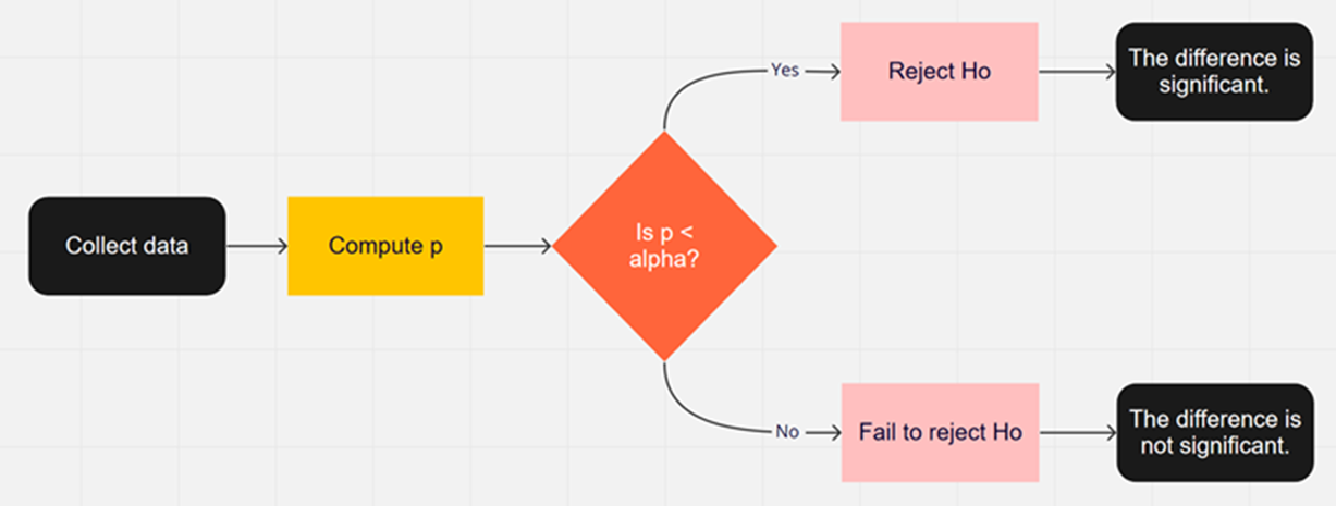
Figure 1: High-level flowchart for statistical hypothesis testing.
Every time you make a binary decision like this, there are two ways to be right and two ways to be wrong.
Consider the example of jury trials from our article about what can go wrong in hypothesis testing. The two ways of being right are by convicting the guilty (analogous to correctly rejecting the null hypothesis and claiming statistical significance) and by acquitting the innocent (correctly failing to reject the null hypothesis for a nonsignificant result).
However, it’s also possible for juries to convict the innocent (concluding a difference is statistically significant when there is no difference; a Type I error or a false positive) or to acquit the guilty (concluding that a difference is not significant when it really is; a Type II error or a false negative).
For any given analysis, you can never know whether the significance decision is correct, but the use of appropriate sample size estimation procedures for hypothesis tests reduces the likelihood of Type I and Type II errors over the long run.
Making a decision about statistical significance is just the first step toward understanding the practical significance of your findings.
Making the Practical Decision from the Statistics
To further interpret the data from the statistical conclusion, we extended the flowchart from Figure 1 by adding further steps to both statistically significant and nonsignificant results, as shown in Figure 2.
1. If the results were statistically significant,
a. Compute a confidence interval around the difference.
b. Interpret the lower limit of the interval to see whether it’s enough to matter.
c. If the lower limit is large enough to matter, it’s practically significant.
2. If the results were NOT statistically significant,
a. Compute a confidence interval around the difference.
b. Are the limits of the confidence interval close to 0?
c. If both limits are close enough to 0, treat the difference as effectively 0 (accepting H0).
d. If both limits are not close enough to 0, the results are ambiguous, so continue to withhold judgment until you have more data.
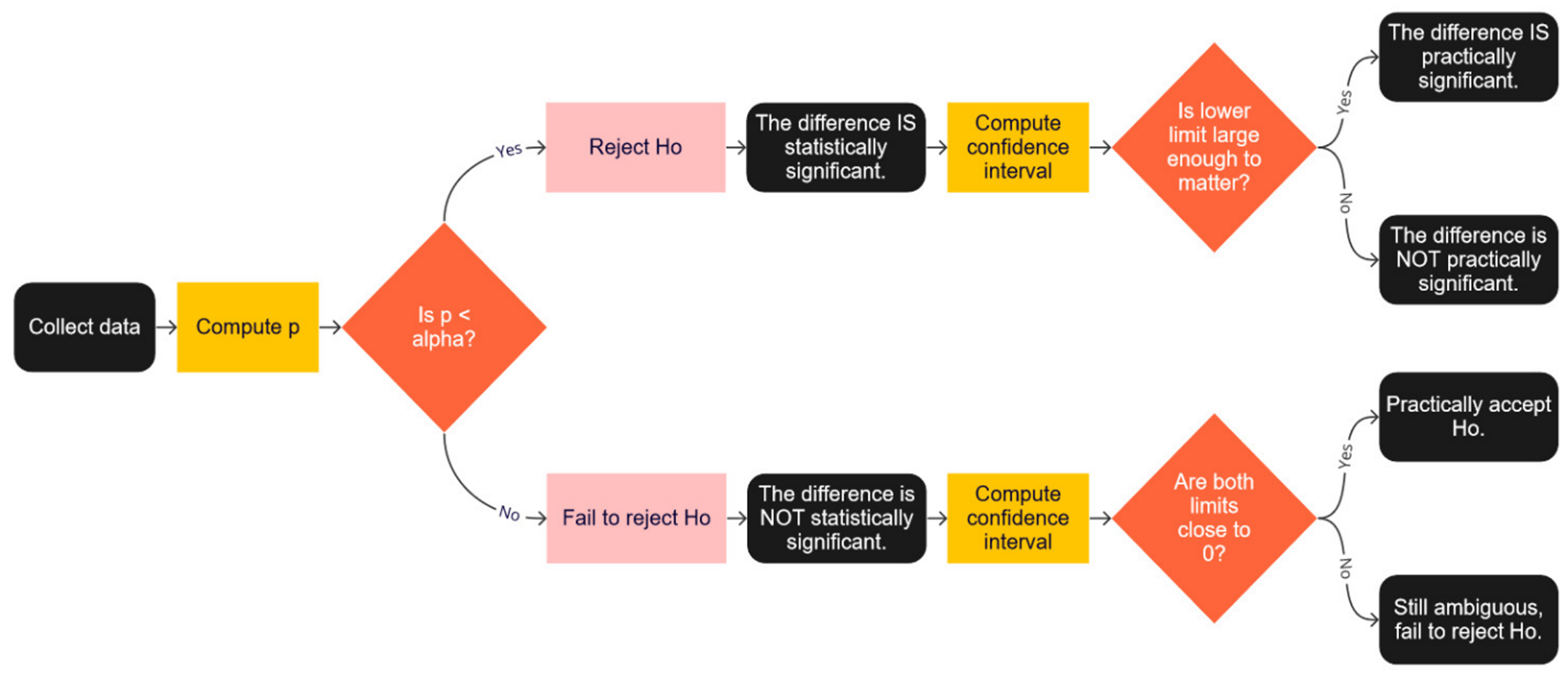
Figure 2: Decision tree for assessing statistical and practical significance.
What Is Large Enough to Matter?
If you can reduce the time it takes a user to complete a task in software by 10 seconds (a statistically significant result), does that matter? It depends. If the 10-second reduction is on a 10-minute task, it’s probably not impactful to the individual user experience. If it’s on a 1-minute task, it probably is. But even a 10-second reduction on a 10-minute task can help a large enterprise; for example, consider a call center that handles a million calls a year.
A small increase in the conversion rate (e.g., .01%) can mean millions of dollars on a website such as Walmart.com. Contexts and judgment always matter, but a good preliminary step to help interpret the potential impact is to compute an effect size. Effect sizes give you some quantitative idea about the size of observed differences expressed in some more universal terms.
To generate a quick effect size, you can take the bounds of the confidence intervals and divide each value by a base to turn it into a percent. For example, reducing a 10-minute task by 10 seconds is a 1.7% reduction (10/600); the same 10-second savings on a 1-minute task is a 17% reduction.
Researchers have to choose which base to use when computing effect sizes. Common choices include the standard deviation of the difference or one of the observed magnitudes from which the difference was computed (typically the larger value—illustrated in the completion time examples above). When a metric has a defined maximum possible difference, you can use that difference can as the base. For example, SUS scores can range from 0 to 100, so the maximum possible difference between two SUS scores is 100 (100 − 0).
For results that are not statistically significant, examine both the lower and upper bounds of the confidence interval to see whether the most extreme value is close enough to 0 to be treated the same as 0 for any practical decision. If so, you can accept H0 because there is no practical difference; if not, the practical result is still ambiguous, so you would continue to withhold judgment pending further investigation.
Decisions about statistical significance are driven mostly by math. Decisions about practical significance are informed by math but driven mostly by professional judgment.
Four Examples of Statistical vs. Practical Significance
When you’re making a small number of comparisons, you could skip the first step (test of significance) and determine significance by whether the confidence interval around the difference includes 0 (not statistically significant) or excludes it (statistically significant). If you need to report the p-value of the test, or if you’re making many comparisons, you should do both steps (test of significance and confidence interval). All the examples assume the conventional criterion of .05.
Example 1: Significant difference (statistically and practically)
After completing five tasks on rental car websites, 14 users completed the System Usability Scale (SUS). The mean SUS scores were 80.4 (sd = 11) for Website A and 63.5 (sd = 15) for Website B, for an observed difference of 16.9. Using the Sauro-Lewis curved grading scale for the SUS to interpret these findings, we found that Website A had an A− and Website B had a C−. Scoring two full grades above Website B was an excellent outcome for Website A.
First step. The result of a dependent-groups t-test was highly significant (t(13) = 3.48, p = .004).
Second step. The 95% confidence interval around the difference ranged from 6.4 to 27.2.
Effect size. Using the maximum possible difference of 100 as a base, we determined that the smallest plausible difference was 6.4%, and the largest plausible difference is 27.2%.
Conclusion. The confidence interval around the difference excluded 0, consistent with the significant t-test. Given the data, the lowest plausible difference was 6.4. If we subtract half of that difference from the observed mean for Website A and add half to Website B, the adjusted means (and associated grades) are, respectively, 77.2 (B+) and 66.8 (C). This result is less impressive than the difference in the observed means but still shows a difference of 1.5 grade levels, which has both practical and statistical significance.
Example 2: Significant difference (statistically but not practically)
We tested two airline websites regarding the ease of booking the best-priced nonstop round-trip ticket. For Airline A, ten users attempted the task, and for Airline B, the sample size was fourteen. Each participant completed the Single Ease Question (SEQ®) after the task. The SEQ is a seven-point item where 1 is “Very difficult” and 7 is “Very easy.” The mean SEQ for Airline A was 6.1 (sd = .83), and for Airline B, it was 5.1 (sd = 1.5), an observed difference of 1.
First step. The outcome of an independent-groups t-test was significant (t(20) = 2.087, p = .0499).
Second step. The 95% confidence interval around the difference ranged from .0005 to 2.0.
Effect size. For a standard seven-point scale, the maximum possible difference is 6 (7 − 1), so the effect sizes of plausible differences ranged from .01% (.0005/6) to 33.3% (2/6).
Conclusion. Consistent with the t-test, the confidence interval did not include 0; given this data, a true difference of 0 was not plausible. On the other hand, a difference as small as .0005 (effect size of one one-hundredth of a percent) was plausible, casting a shadow on the practical significance of the result.
Example 3: Nonsignificant difference (fail to reject H0)
We conducted a test between two CRM applications. Eleven users attempted tasks on Product A, and twelve different users attempted the same tasks on Product B. Product A had a mean SUS score of 51.6 (sd = 4.07), and Product B had a mean SUS score of 49.6 (sd = 4.63), an observed difference of 2.
First step. An independent group’s t-test found this difference was not statistically significant (t(20) = 1.1, p = .28).
Second step. The 95% confidence interval around the difference ranged from −1.8 to 5.8.
Effect size. Using the maximum possible difference of 100 as a base, we determined the effect size range as −1.8% to 5.8%.
Conclusion. The confidence interval contained 0, so the null hypothesis of no difference is plausible (consistent with the nonsignificant t-test). The bounds of the confidence interval showed that differences as extreme as −1.8 and 5.8 were also plausible. Therefore, the outcome is too ambiguous to draw any practical conclusions.
Example 4: Nonsignificant difference (practically accept H0)
In a survey of UX measures of streaming video services, 240 respondents completed two versions of the UMUX-Lite, one with numeric scale points and one with face emojis (with appropriate counterbalancing). The mean for the numeric version was 85.9 (sd = 17.5), and for the face emojis version, it was 85.4 (sd = 17.1), a difference of a half-point on a 0-100–point scale.
First step. A dependent-groups t-test indicated the difference was not statistically significant (t(239) = .88, p = .38).
Second step. The 95% confidence interval around the mean ranged from −.6 to 1.5.
Effect size. Like the SUS, the maximum possible UMUX-Lite difference is 100, so the effect size ranged from −.6% to 1.5%.
Conclusion. Consistent with the t-test, the confidence interval contained 0 (null hypothesis is plausible). Examination of the upper and lower bounds of the interval showed that the largest plausible difference was 1.5. When the largest plausible difference is small enough, it’s effectively 0 for purposes of decision-making. Even though you can’t formally accept the null hypothesis, you can effectively accept it for practical purposes.
Summary
With statistical hypothesis testing, you make decisions never knowing whether you’ve made a Type I or Type II error for any specific decision, but by using this method, you limit the likelihood of those errors over the long run.
Making a decision about statistical significance is just the first step. Another “error” you can make when using statistical hypothesis testing, especially in business and industrial applications (as opposed to critical experiments that test scientific theories), is to stop after the assessment of statistical significance without also assessing practical significance.
One way to move beyond statistical significance testing is by examining confidence intervals constructed around observed differences and considering the associated effect sizes. Some statistically significant results may turn out to have limited practical significance, and some results that are not statistically significant can lead to practical acceptance of the null hypothesis of no difference.


