 We recently described how to compare two Net Promoter Scores (NPS) statistically using a new method based on adjusted-Wald proportions.
In addition to comparing two NPS, researchers sometimes need to compare one NPS with a benchmark.
For example, suppose you have data that the average NPS in your industry is 17.5%, and you want to know whether your NPS of 20% is significantly above that average. Or maybe you may want to determine if your NPS exceeds 50%, a benchmark considered “excellent” by some for the introduction of new products.
In this article, we show how to modify the method for comparing two NPS into a method that will allow you to compare a single NPS with a benchmark. We will also show how to compute an appropriate confidence interval.
Benchmark-Testing the NPS
Special considerations for benchmark testing
Most statistical comparisons of two estimated values use a strategy known as two-tailed testing. The term “two-tailed” refers to the tails of the distribution of the differences between the two values. The left distribution in Figure 1 illustrates a two-tailed test showing the rejection criterion (α = .05) evenly split between the two tails.
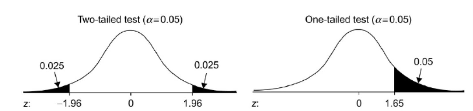
Figure 1: One- and two-sided rejection regions for one- and two-sided significance tests.
When you test an estimated value against a benchmark, you care only that your estimate is significantly better than the benchmark. When that is the case, you can conduct a one-tailed test, illustrated by the right distribution in Figure 1. Instead of splitting the rejection region between two tails, it’s all in one tail. The practical consequence is that the bar for declaring significance is lower for a one-tailed test (Z > 1.645 vs. |Z| > 1.96).
Computational details
Here are the computational details for the test with a fully worked-out example. Note that to keep computations as simple as possible, we usually work with the NPS as proportions and convert to percentages only when reporting scores.
To use this method, you need to know the number of detractors, passives, and promoters for the estimated NPS (usually available in company dashboards). The computational steps are
- Add 3 to the sample size: n.adj = n + 3.
- Add ¾ to the number of detractors: ndet.adj = ndet + ¾.
- Add ¾ to the number of promoters: npro.adj = npro + ¾.
- Compute the adjusted proportion of detractors: pdet.adj = ndet.adj/n.adj.
- Compute the adjusted proportion of promoters: ppro.adj = npro.adj/n.adj.
- Compute the variance: Var.adj = ppro.adj + pdet.adj − (ppro.adj − pdet.adj)2.
- Compute the adjusted NPS: NPS.adj = ppro.adj − pdet.adj.
- Compute the difference between the adjusted NPS and the target benchmark: NPS.diff = NPS.adj − Benchmark.
- Compute the standard error of the difference: se.diff = (Var.adj/n.adj)½.
- Divide the difference by the standard error to get a Z score: Z = NPS.diff/se.diff.
- Assess the significance of the difference by getting the one-tailed p-value for Z; in Excel, you can use the formula: =1-NORM.S.DIST(Z,TRUE).
For example, in a UX survey of an email application conducted in early 2020, we collected likelihood-to-recommend ratings from 107 respondents. The estimated NPS was 42% (61 promoters, 30 passives, and 16 detractors; so ppro = 61/107 = .570 and pdet = 16/107 = .150). Table 1 shows the steps to compute the significance of this estimate (41% after adjustment) with three benchmarks—one small difference (Benchmark = 40%; difference = 1%), one moderate difference (Benchmark = 30%; difference = 11%), and one relatively large difference (Benchmark = 20%; difference = 21%).
| Compute NPS and Variance | n.adj | ppro.adj | pdet.adj | NPS.adj | Var.adj |
|---|---|---|---|---|---|
| Email Application | 110 | 0.56 | 0.15 | 0.41 | 0.546 |
| Benchmark Test | NPS.diff | se.diff | Z | p(Z) |
|---|---|---|---|---|
| NPS = 40% | 0.01 | 0.070 | 0.129 | 0.449 |
| NPS = 30% | 0.11 | 0.070 | 1.548 | 0.061 |
| NPS = 20% | 0.21 | 0.070 | 2.967 | 0.002 |
Table 1: Assessing the significance of differences between an estimated NPS and three benchmarks.
As shown in Table 1, the test was not significant (p = .449) when the difference between the estimated NPS and the benchmark was small relative to the standard error. In other words, the evidence doesn’t support the hypothesis that the observed NPS has exceeded the benchmark. When the difference was large relative to the standard error, the outcome was statistically significant (p = .002). For the more moderate difference, the outcome (p = .061) just missed p < .05 (but was significant at p < .10).
Constructing a Confidence Interval for a One-Tailed Test of NPS
A test of significance is often a reasonable first step in an analysis, but it has limited utility for assessing the practical significance of the result. For that, you need a confidence interval. Because we’re interested in only the lower limit of the interval exceeding the benchmark, set the confidence level to 1 − 2α, where α is the rejection criterion for the test of significance. (For example, if you plan to claim significance when p < .05, then the rejection criterion α is equal to .05.) The steps for constructing an appropriate adjusted-Wald confidence interval are
- Find Z for the desired level of confidence: For one-sided tests, common values are 1.645 for 95% confidence and 1.282 for 90% confidence.
- Compute the margin of error for the interval: MoE = Z(se.diff).
- Compute the confidence interval around the adjusted NPS: NPS.adj ± MoE.
Table 2 shows the resulting 95% confidence interval, and Figure 2 shows a graph of the adjusted-Wald interval around the unadjusted NPS.
| Product | NPS.adj | Std Error | Z95 | MoE95 | Lower95 | Upper95 |
|---|---|---|---|---|---|---|
| Email Application | 0.41 | 0.070 | 1.645 | 0.116 | 0.29 | 0.53 |
Table 2: One-sided 95% adjusted-Wald confidence interval around the estimated NPS.
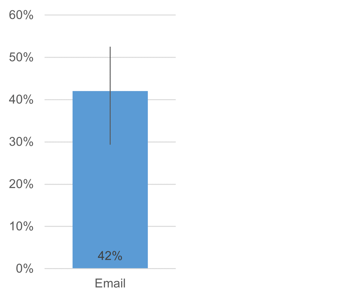
Figure 2: Graph of the 95% adjusted-Wald confidence interval around the estimated NPS.
The interval ranges from 29% to 53%, so if any proposed benchmark falls within this range, it could plausibly be equal to the observed NPS. Because this data is associated with a one-sided test and we care only about beating a benchmark, we can conclude that the observed NPS is significantly higher than any benchmark lower than its lower limit of 29% with p < .05 (consistent with the results in Table 1). Strictly speaking, we can’t draw any conclusions about the upper limit of this one-sided interval.
Summary
Sometimes UX researchers need to compare an estimated NPS with a benchmark (such as an NPS of 50%), not compare two NPS from sample data (e.g., comparing Q1 vs. Q2 scores).
We’ve worked out methods for making NPS benchmark comparisons with a test of significance and/or an appropriate confidence interval.
Both analyses (significance testing and confidence interval) use adjusted-Wald proportions, which previous research has shown to be the best approach when working with NPS. In this case, using the adjusted-Wald means modifying the observed data by adding 3 to the total sample size, ¾ to the number of detractors, and ¾ to the number of promoters.
One special consideration for benchmark evaluation is to use one-tailed instead of a two-tailed test to increase measurement sensitivity.


