 We’ve written a lot about confidence intervals for the last two decades.
We especially encourage them for small sample studies.
Some of you even bought into our recommendation and use them yourselves (a decision we continue to support).
But maybe you’ve heard about Bayesian credible intervals and wonder if you should be using them instead.
In this article, we return to an example used in our previous articles on Bayesian methods applied to UX research and compare analyses of that example with confidence and credible intervals.
Confidence Interval Analysis
In our recurring example, 18 of 20 participants successfully completed a checkout task (a 90% completion rate). But if we were to test hundreds, thousands, or (somehow) all potential users, would the completion rate be exactly 90%? Almost surely not. But instead of trying to nail down an exact single number, a likely range is usually sufficient for decision making and surprisingly easy to compute and accurate even for small sample sizes.
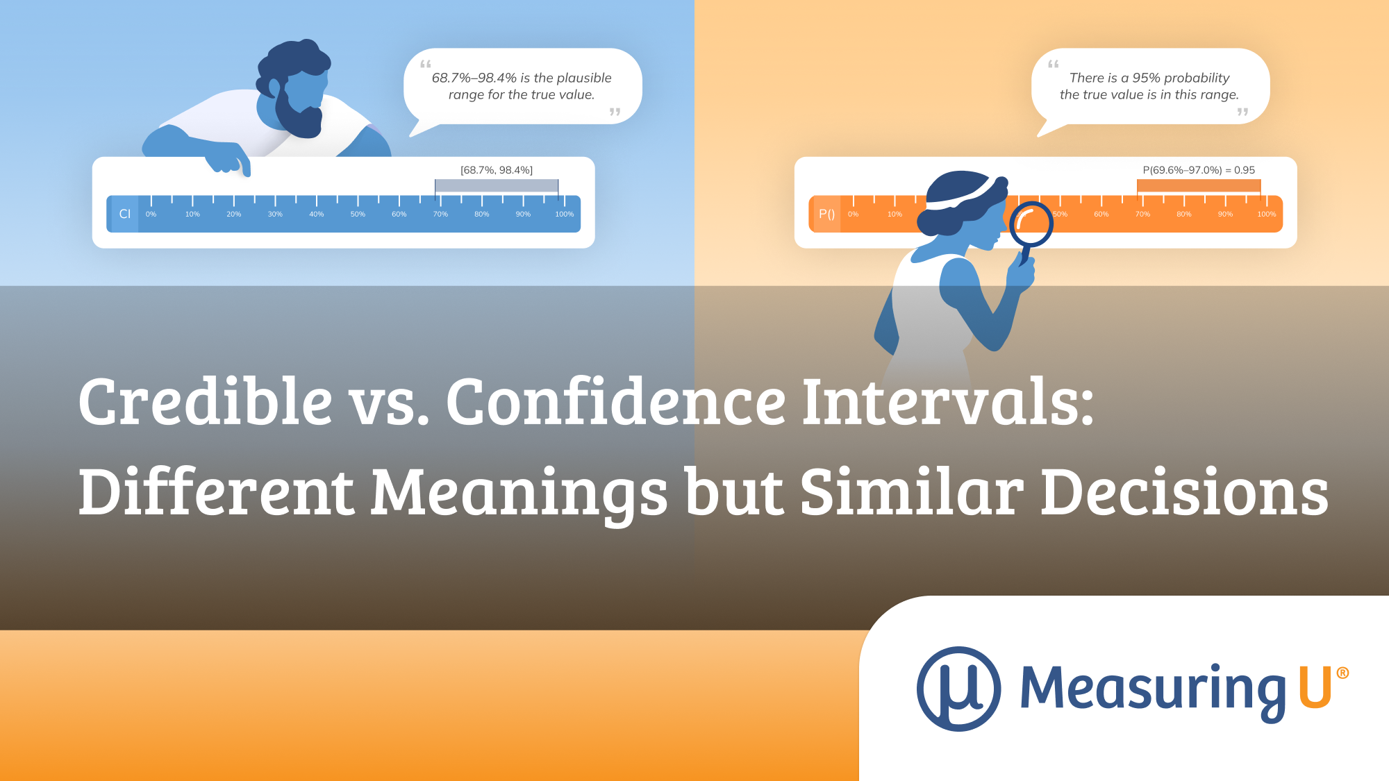
For this type of data (binary), the likely range can be computed using an adjusted-Wald confidence interval with 95% confidence. That interval is 68.7% to 98.4%.
We’ve made it easy to compute binomial confidence intervals with our online calculator. But how do you interpret or explain what it means? How about:
- There’s a 95% probability the true completion rate is between 68.7% and 98.4%.
- There’s a 95% chance the true completion rate falls within 68.7% and 98.4%.
- 95% of future tests with completion rates will be between 68.7% and 98.4%.
Strictly speaking, all three of those statements are wrong. A stats professor or Bayesian enthusiast will be happy to point out that error.
The more technically correct way to describe the interval is:
- If we ran many tests, each with 20 users from the same population and computed confidence intervals each time, on average, 95 out of 100 confidence intervals will contain the unknown population completion rate.
Strictly speaking, we are 95% confident in the method of generating confidence intervals and not in any given interval. The confidence interval we generated from the sample data either does or does not contain the population completion rate.
We don’t know if our sample of 20 is one of those five whose confidence interval doesn’t contain the completion rate. So, it’s best to avoid using “probability” or “chance” when describing a confidence interval and remember that we’re 95% confident in the process of generating confidence intervals rather than a given interval.
So, we have just one study, and we computed only one interval. What does that mean? What are we “allowed” to say other than that cumbersome statement? We have a couple of recommendations suitable for practical decision making:
- Likely range: “68.7% to 98.4% is the most likely range for the unknown completion rate from all users.”
- Plausible range (from Smithson, 2002): “Given this data, values inside the confidence interval are plausible while those outside are implausible. The observed completion rate of 90% is plausible but rates lower than 68.7% or higher than 98.4% are implausible.”
This is where the precision of numbers meets the imprecision of language. Although confidence, probability, likely, and plausible all sound about the same, they have more precise usage when it comes to statistics and probability.
This rigidity in language makes them less ideal when communicating the results to stakeholders who will not likely have a sophisticated understanding of confidence intervals (although even professors sometimes struggle with the concept).
Credible Interval Analysis
One proposed alternative is the Bayesian credible interval.
Credible intervals are designed to allow for the interpretation people naturally want to use. A 95% credible interval can be interpreted as having a 95% probability of containing the true value.
Like with confidence intervals, there are different computations used to generate credible intervals on binary data. And like with confidence intervals, there are debates about which method is optimal. We won’t get into that debate here. Instead, we’ve provided in Table 1 three Bayesian credible intervals for our example that differ in their priors (all of which are commonly used in practice).
| Method | Prior/Setup | 95% Interval |
|---|---|---|
| Adjusted-Wald | Add ~2 successes & ~2 failures | 68.7% to 98.4% |
| Bayesian credible interval | Beta(1,1)—Uniform prior | 69.6% to 97.0% |
| Bayesian credible interval | Beta(0.5, 0.5)—Jeffreys prior | 71.6% to 97.9% |
| Bayesian credible interval | Beta(2, 2)—Agresti prior | 66.4% to 95.0% |
Table 1: Four 95% interval estimates, one confidence and three credible.
For example, a 95% Bayesian credible interval using a uniform prior for 18 successes and 2 failures generates a credible interval of 69.6% to 97.0%.
We can say there’s a 95% probability that the true and unknown completion rate is between 69.6% and 97%.
Stats professors are happy with that statement. Bayesian purists are happy with that statement. And your stakeholders probably understand that statement too!
So, should we all start using credible intervals and abandon confidence intervals? Not necessarily.
Credible intervals require more complex calculations and usually don’t have the simple closed-form solution of the adjusted-Wald interval. In practice, however, this difference is negligible because modern software handles the computation (e.g., we used the binom.bayes function in the R package binom).
But did you notice anything about the values in Table 1? The intervals are all very similar, as shown in the graph in Figure 1.

Figure 1: Graph of the four intervals (Green: adjusted-Wald, Blue: Bayesian Uniform, Orange: Bayesian Jeffreys, Black: Bayesian Agresti); dashed green line shows limits of adjusted-Wald interval across the three Bayesian intervals.
There are very few differences between the intervals. The width of the adjusted-Wald interval is 29.7%. The Uniform and Jeffreys intervals lie within the adjusted-Wald (with respective widths of 27.4% and 26.3%) while the Agresti interval has about the same width as the adjusted-Wald (28.6%), with its upper and lower endpoints shifted down relative to the adjusted-Wald interval by, respectively, 3.4% and 2.3%.
If the output is roughly the same, does it really matter? The numbers don’t know where they come from.
This is similar to the debate about ordinal versus interval data. As Lord (1951) noted, even nominal values like football jersey numbers can be averaged. The math works, but proper interpretation is critical.
Confidence intervals and credible intervals can yield nearly identical results, especially for this type of data. In many cases, they will lead to the same practical decision, even though the interpretation differs.
So, what should you do?
The results here suggest that, at least for this type of data, traditional confidence intervals and Bayesian credible intervals can produce very similar ranges. The main difference is not in the numbers, but in how we interpret and communicate them.
That’s one reason we continue to recommend confidence intervals. They are well understood, widely taught, and, when used appropriately, provide accurate estimates of the range of plausible values.
At the same time, we understand the appeal of credible intervals. The interpretation is more natural and often aligns better with how stakeholders think about uncertainty.
In practice, either approach can be effective. What matters most is understanding what the interval represents and communicating it clearly. Decisions are made by inspecting the endpoints of the intervals. If you’d make the same decision for both endpoints, then you have enough information to make the decision. Otherwise, you need more data. In this example, it seems unlikely that the slight variation in endpoint values would affect real-world decision making.
Notably, in this example, the confidence interval encompassed two of the Bayesian intervals, so not only did it have 95% confidence from a frequentist perspective, but it also had at least 95% credibility from a Bayesian perspective.
We’ll continue to explore where these approaches differ more meaningfully in future articles, including whether these similarities extend beyond this example to different proportions and to other statistics such as means.
Key Takeaways
In this latest article on Bayesian methods, we covered:
- Confidence intervals are harder to explain than most people think.
- Credible intervals match how people want to interpret uncertainty.
- In this example, both methods produce very similar ranges.
- The difference is less about the numbers and more about what we can say about them.
- Use either approach thoughtfully, but focus on clear communication.