“That confirms what I expected.”

The same data, two different conclusions.

A 90% completion rate from 20 participants on a usability test of a checkout flow. Is that completion rate better than the historical average of 78%?

One researcher says yes, definitely. Another says no, it’s in line with the historical average.

Both are using the same Bayesian method. How can the same data produce opposite conclusions?

The answer lies in priors, the assumptions you bring to the analysis before the data impact the decision.

In our previous article, we assumed equal priors when analyzing completion rate data to simplify the analysis. But what happens when those priors change?

In this article, we explore the consequences of manipulating those prior probabilities in different ways.

The Effect of Priors on the Outcome

In Bayesian analysis, we assign numerical probabilities to prior beliefs about competing hypotheses. Priors reflect how plausible we think each explanation is before seeing the current data.

If a prior belief is well supported, we give it more weight. If it’s less credible, we give it less weight. When we don’t have strong prior information, we can assign roughly equal weights, allowing the observed data to play a larger role in the conclusion.

In our example, 18 of 20 participants successfully completed a task (a 90% completion rate). We want to understand how different prior beliefs affect our interpretation of this result when compared to a historical completion rate of 78%.

To do this, we compare two hypotheses: that the true completion rate is 78% (historical) or 90% (based on the observed data), under different prior assumptions. We could also test other values (e.g., 85% or 95%), but we use 90% as a convenient reference based on the sample, recognizing that this is a simplifying modeling choice.

So, which is more plausible: a 78% or 90% completion rate?

We examine five scenarios that vary the strength and direction of the prior belief:

1. Neutral prior (no preference)
2. Weak prior favoring a 78% completion rate
3. Weak prior favoring a 90% completion rate
4. Strong prior favoring a 78% completion rate
5. Strong prior favoring a 90% completion rate

So how do we quantify the strength of our prior beliefs? What values should we use to represent neutral, weak, and strong preferences for one hypothesis over another?

A neutral prior is straightforward, a 50/50 reflecting no preference. But once we move beyond that, the choice of “weak” or “strong” priors becomes less clear.

If we move slightly off a neutral stance, values like 60/40 seem reasonable. But whether we use 60/40, 70/30, or 80/20 is somewhat arbitrary. We use 0.6 and 0.8 to represent weak and strong prior preferences, respectively.

To avoid confusion between completion rates (e.g., 90%) and prior probabilities (e.g., 0.8), we use decimal values for the priors.

When we apply these values to the Bayesian formula (see the appendix), we obtain the results shown in Table 1.

Each row represents a different prior scenario. The second and third columns show the prior beliefs assigned to each hypothesis. The next two columns show how those beliefs are updated after observing 18 of 20 participants complete the task. The final column shows the relative likelihood of the two hypotheses.

For example, with neutral priors, the 90% completion rate is 2.7 times more likely than the 78% completion rate. In contrast, with a strong prior favoring 78%, the 78% completion rate becomes more likely than the 90% completion rate.

Prior Scenario	Prior Belief in		Updated Belief in		Which Is More Likely?	Odds (90% vs. 78%)
	90%	78%	90%	78%
Neutral prior (no preference)	0.5	0.5	0.732	0.268	90%	2.7×
Weak prior favoring 78%	0.4	0.6	0.645	0.355	90%	1.8×
Weak prior favoring 90%	0.6	0.4	0.804	0.196	90%	4.1×
Strong prior favoring 78%	0.2	0.8	0.405	0.595	78%	0.68× (≈1.5× for 78%)
Strong prior favoring 90%	0.8	0.2	0.916	0.084	90%	10.9×

Table 1: Effect of different priors on updated beliefs.

How Our Conclusions Change Based on Priors

Across all five scenarios, a 90% completion rate is more likely in four of them. In one case, it’s more than ten times as likely as the 78% completion rate. Only when we strongly favor the historical data does the conclusion shift, making the 78% completion rate more likely despite the observed results.

Changing only the prior belief can shift the conclusion from favoring 78% to strongly favoring 90%. No new data were added. In this example, changing the prior assumption had a larger effect on the conclusion than a modest increase in sample size would. This raises a natural question: how much additional data would be needed to overcome a strong prior?

This highlights an important property of Bayesian analysis. The conclusions are influenced not only by the observed data, but also by the strength and direction of the prior beliefs. When priors are strong, they can reinforce or counteract the data. When priors are weak or neutral, the data play a larger role.

Who decides what the historical data is and how relevant it is? And how strongly do you weight the priors? There isn’t a Bayesian rule book we can reference. Instead, it comes down to making informed and good judgments. But is that judgment always clear, and does it lead to better conclusions?

Understanding how priors affect the decision (under one scenario) is the easy part. Teasing out the pros and cons of this approach with more Bayesian methods and real-world scenarios is the harder one. And the subject of some upcoming articles.

This illustrates both the potential power and the potential risk of Bayesian analysis. It can incorporate prior knowledge in a principled way, but when priors are uncertain, subjective, or weakly supported, the results may reflect assumptions as much as evidence.

Summary and Discussion

In a previous article, we extended a classical problem in Bayesian comparison of the likelihoods of two hypotheses to a UX research context using an approach that required only simple algebra.

In this article, we showed how variation in prior belief can affect the posterior likelihoods of competing UX hypotheses, potentially having a larger impact than small changes in the observed data. For this example, varying the priors had a large effect on the likelihoods of the hypotheses (from 0.405 to 0.916 for the 90% hypothesis). This may, in part, have been affected by the relatively small difference in the competing hypotheses (78% vs. 90%, just a 12-point difference).

What Should Researchers Do About Priors?

In practice, researchers should:

• Be explicit about the priors they use and how they were chosen.
• Test multiple plausible priors to understand how sensitive the conclusions are to variation in priors (e.g., prior sensitivity analysis).
• Be cautious when priors are uncertain or weakly supported.
• Consider collecting more data when conclusions depend heavily on prior assumptions.

Understanding how priors influence results is an important step in using Bayesian methods effectively. It does not mean avoiding Bayesian analysis, but it does mean using it thoughtfully and transparently.

Appendix

For this example, we assumed 20 participants attempted an online checkout task with 18 successes and 2 failures (90% success). With that result, we want to understand whether it’s more likely that the true successful completion rate is 78% (historical) or our observed 90% (better than historical).

To get the odds ratios displayed in Table 1, we used the following Bayesian formula.

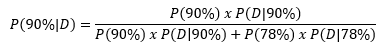
where:

P(D|90%) is the probability of getting this sample (the data, D) if the true completion rate is 90%.

P(D|78%) is the probability of getting this sample if the true completion rate is 78%.

P(90%) is our expected (prior) probability that the true completion rate is 90%.

P(78%) is our expected (prior) probability that the true completion rate is 78%.

P(90%|D) is the conditional probability of the completion rate being 90% given the sample.

P(78%|D) is 1 – P(90%|D).

Using the binomial probability formula, we can compute the probabilities of getting this sample for each of the hypothesized true completion rates:

P(D|90%) is (0.9)¹⁸ × (0.1)² = 0.0015.

P(D|78%) is (0.78)¹⁸ × (0.22)² = 0.00055.

Next, we apply this formula to the five sets of priors (Neutral, Weak Favoring 78%, Weak Favoring 90%, Strong Favoring 78%, Strong Favoring 90%).

Technical note: We used binomial probabilities throughout this article because they allow us to illustrate the mechanics of the Bayesian analyses with simple algebra. The downside of this simplification is that we had to assign specific prior probabilities rather than using the current practice of using beta distributions for priors, but this does not affect the logic of the discussion. Also, we excluded the factorial component of the binomial probability formula because it was constant across the computations.

Neutral Prior

If we decide there is no basis for weighting the priors unequally, the values for the formula are:

P(90%) = 0.5

P(78%) = 0.5

P(D|90%) = 0.0015

P(D|78%) = 0.00055

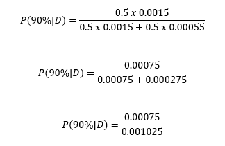
So:

P(90%|D) = 0.732

P(78%|D) = 0.268

P(90%|D) / P(78%|D) = 2.73

P(78%|D) / P(90%|D) = 0.37

Conclusion: There is a substantial likelihood that the historical hypothesis (78%) might be true (0.268 isn’t anywhere near 0), but the alternative hypothesis (90%) is 2.7 times more likely.

Weak Prior Favoring 78%

If we decide to give a little more weight to the historical hypothesis (78%) and a little less to the alternative hypothesis (90%), we get:

P(90%) = 0.4

P(78%) = 0.6

P(D|90%) = 0.0015

P(D|78%) = 0.00055

So:

P(90%|D) = 0.645

P(78%|D) = 0.355

P(90%|D) / P(78%|D) = 1.82

P(78%|D) / P(90%|D) = 0.55

Conclusion: There is a substantial likelihood that the historical hypothesis (78%) might be true (0.355 isn’t anywhere near 0), but the alternative hypothesis (90%) is 1.8 times more likely.

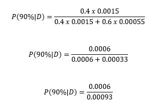
Weak Prior Favoring 90%

If we decide to give a little more weight to the alternative hypothesis (90%) and a little less to the historical hypothesis (78%), we get:

P(90%) = 0.6

P(78%) = 0.4

P(D|90%) = 0.0015

P(D|78%) = 0.00055

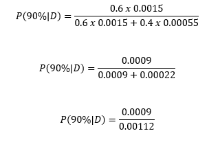
So:

P(90%|D) = 0.804

P(78%|D) = 0.196

P(90%|D) / P(78%|D) = 4.09

P(78%|D) / P(90%|D) = 0.24

Conclusion: There is a decent likelihood that the historical hypothesis (78%) might be true (0.196 isn’t that close to 0), but the alternative hypothesis (90%) is 4.1 times more likely.

Strong Prior Favoring 78%

If we decide to give a lot more weight to the historical hypothesis (78%) and a lot less to the alternative hypothesis (90%), we get:

P(90%) = 0.2

P(78%) = 0.8

P(D|90%) = 0.0015

P(D|78%) = 0.00055

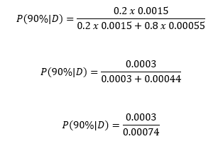
So:

P(90%|D) = 0.405

P(78%|D) = 0.595

P(90%|D) / P(78%|D) = 0.68

P(78%|D) / P(90%|D) = 1.47

Conclusion: The historical hypothesis (78%) is about 1.5 times more likely than the alternative hypothesis (90%), but not by much (both likelihoods aren’t that far from 50%).

Strong Prior Favoring 90%

If we decide to give a lot more weight to the alternative hypothesis (90%) and a lot less to the historical hypothesis (78%), we get:

P(90%) = 0.8

P(78%) = 0.2

P(D|90%) = 0.0015

P(D|78%) = 0.00055

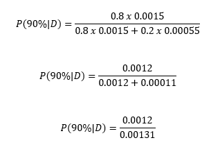
So:

P(90%|D) = 0.916

P(78%|D) = 0.084

P(90%|D) / P(78%|D) = 10.91

P(78%|D) / P(90%|D) = 0.09

Conclusion: There is relatively little likelihood that the historical hypothesis (78%) might be true (0.084 is getting close to 0), and the alternative hypothesis (90%) is 10.9 times more likely.