
The Net Promoter Score (NPS) is a widely used metric, but it can be tricky to work with statistically.
One of the first statistical steps we recommend that researchers take is to add confidence intervals around their metrics. Confidence intervals provide a good visualization of how precise estimates from samples are. They are particularly helpful in longitudinal research to help differentiate the inevitable fluctuations in data from sampling error with meaningful changes that often need further investigation.
But until recently, there was no well-defined method for computing NPS confidence intervals.
The NPS uses a single likelihood-to-recommend (LTR) question (“How likely is it that you would recommend our company to a friend or colleague?”) with 11 scale steps from 0 (Not at all likely) to 10 (Extremely likely). A confidence interval can be computed on the mean LTR score using a well-known method for rating scales, but this approach doesn’t account for how the NPS is computed. In NPS terminology, respondents who select 9 or 10 on the LTR question are “Promoters,” those selecting 0 through 6 are “Detractors,” and all others are “Passives.” The NPS is the percentage of Promoters minus the percentage of Detractors (the “net” in “Net Promoter”).
The developers of the NPS hold that this metric is easy for managers to understand and to use to track changes over time, and research has shown the NPS has a strong relationship to company growth and actual recommendation behavior.
If you do a web search for ways to compute NPS confidence intervals, you’ll find plenty of suggestions with no supporting research on the accuracy of the resulting intervals. A major exception is an excellent paper published by Brendan Rocks (2016) in The American Statistician. To evaluate the quality of six methods for computing NPS confidence intervals, he investigated their precision and coverage for samples drawn from theoretical trinomial distributions and from over a thousand NPS distributions based on real-world data.
The precision of a confidence interval is its width: narrower intervals are better than wider intervals. The coverage of a method for computing confidence intervals is the percentage of times in iterative resampling that the computed interval contains the true value of the estimated statistic (in this case, the NPS computed from the entire dataset sample), which should be close to the stated confidence level. In other words, if you’ve set confidence to 95%, then you expect the interval to contain the target value 95% of the time. Of these quality metrics, coverage is more important than precision.
Rocks’ key finding was that the best-performing method for constructing NPS confidence intervals was a variant of the adjusted-Wald method, designated (3, T). We first encountered adjusted-Wald methods in 2005 when we found it to be the best way to compute binomial confidence intervals (which is why it’s the most prominent method in our online confidence interval calculator for completion rates).
Adjusted-Wald methods work by adding values to observed counts. For a binomial confidence interval, you need to look up the Z-value for the desired level of confidence (e.g., 1.96 for 95% confidence) and then add Z2/2 to the numerator and Z2 to the denominator before using the Wald method to compute the confidence interval. See Chapter 3 in Quantifying the User Experience for more details on the adjusted-Wald interval for binary data.
Applying this concept to the NPS, Rocks found that the best adjustment method was to add a constant of 3 to the sample size (n), ¾ to the number of detractors, and ¾ to the number of promoters, and then compute the interval using a standard error based on the variance of the difference in two proportions.
We decided to try Rocks’ adjusted-Wald method for ourselves, comparing it to two other procedures that he didn’t include in his research—a Means method and a bootstrapping method.
Three Methods for Computing Confidence Intervals for NPS
Here are details about the three methods we explored for computing NPS confidence intervals. Note that to keep computations simple in this section, we worked with NPS as proportions and converted to percentages.
Adjusted-Wald (3, T)
To use this method, you need to know the number of detractors, passives, and promoters. The computational steps are
- Add 3 to the sample size: n.adj = n + 3.
- Add ¾ to the number of detractors: ndet.adj = ndet + ¾.
- Add ¾ to the number of promoters: npro.adj = npro + ¾.
- Compute the adjusted proportion of detractors: pdet.adj = ndet.adj/n.adj.
- Compute the adjusted proportion of promoters: ppro.adj = npro.adj/n.adj.
- Compute the variance: Var.adj = ppro.adj + pdet.adj − (ppro.adj – pdet.adj)2.
- Compute the adjusted NPS: NPS.adj = ppro.adj − pdet.adj.
- Compute the adjusted standard error: se.adj = (Var.adj/n.adj)1/2.
- Look up the Z-value for the desired level of confidence (e.g., for 90% confidence, Z = 1.645).
- Compute the margin of error: MoE = Z(se.adj).
- Compute the upper and lower bounds of the confidence interval: NPS.adj ± MoE.
For example, in a UX survey of online meeting services conducted in 2019, we collected likelihood-to-recommend ratings. For GoToMeeting (GTM), there were 8 detractors, 13 passives, and 15 promoters, for an NPS of 19% (n = 36). For WebEx, there were 12 detractors, 12 passives, and 7 promoters, for an NPS of -16% (n = 31). Table 1 shows the steps to compute their 90% confidence intervals.
| Service | n.adj | ppro.adj | pdet.adj | NPS.adj | Var.adj | se.adj | z90 | MoE90 | Lower90 | Upper90 |
|---|---|---|---|---|---|---|---|---|---|---|
| GTM | 39 | 0.40 | 0.22 | 0.18 | 0.596 | 0.124 | 1.645 | 0.203 | −0.02 | 0.38 |
| WebEx | 34 | 0.23 | 0.38 | −0.15 | 0.581 | 0.131 | 1.645 | 0.215 | −0.36 | 0.07 |
Table 1: Computing 90% adjusted-Wald confidence intervals for the NPS of two online meeting services.
Means
For this method, you need to have data for each response to the likelihood-to-recommend item, assigning −1 to detractors, 0 to passives, and +1 to promoters. The computational steps are
- Compute the sample mean and standard deviation(s).
- Compute the standard error: s/(n1/2).
- Look up the t-value for the desired confidence level and degrees of freedom (df = n−1).
- Compute the margin of error: MoE = t(se).
- Compute the confidence interval: mean ± MoE.
Note that this method is the same t-based interval used on rating scale data, but instead of using the full 11 points of the LTR, it’s computed using the three-point NPS trinomial (−1, 0, 1).
Table 2 shows the computational steps and results for the GTM and WebEx data:
| Statistic | GTM | WebEx |
|---|---|---|
| Mean | 0.19 | −0.16 |
| St Dev | 0.79 | 0.78 |
| N | 36 | 31 |
| se | 0.131 | 0.140 |
| df | 35 | 30 |
| tcrit90 | 1.690 | 1.697 |
| MoE90 | 0.221 | 0.237 |
| Upper90 | 0.42 | 0.08 |
| Lower90 | −0.03 | −0.40 |
Table 2: 90% confidence intervals for two online meeting services using the Means method.
Bootstrapping
Bootstrapping is a nonparametric distribution-free method for computing confidence intervals. For this method, you need to have data for each response to the likelihood-to-recommend item, assigning −1 to detractors, 0 to passives, and +1 to promoters. The computational steps are:
- With replacement, draw a random sample from the observed sample equal to its sample size.
- Compute the mean of the random sample.
- Save this mean.
- Iterate steps 2 and 3 at least a thousand times.
- Sort the saved means from smallest to largest.
- For the desired confidence level, identify the values toward the lower and upper ends of the distribution between which the proportion of means matches the desired confidence (for a 90% interval, these would be the values at the 5th and 95th percentiles).
- These values are the lower and upper bounds of the bootstrap confidence interval.
Due to the large number of iterations required to build up the empirical distribution, it’s necessary to use computers. For this evaluation, we used the bootstrapping function available in SPSS. Applying it to the GTM and WebEx data, we got the following 90% bootstrap confidence intervals:
- GTM: −.03 to .42
- WebEx: −.40 to .08
Comparing the Methods
Table 3 shows the 90% interval widths (precision) for each of the three methods, in descending order. See Figure 1 for a graph of the confidence intervals.
| Method | GTM | WebEx | Average |
|---|---|---|---|
| Means | 0.44 | 0.47 | 0.46 |
| Bootstrap | 0.43 | 0.46 | 0.45 |
| Adj Wald | 0.40 | 0.43 | 0.42 |
Table 3: 90% confidence interval widths for the three methods.
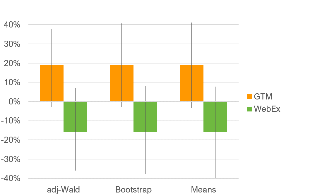
Figure 1: 90% confidence intervals for both services and the three methods.
All three methods produced intervals with similar location and precision. To our surprise, the simple Means approach produced intervals that were not dramatically wider than those generated with the more sophisticated methods. However, consistent with the findings of Rocks (2016), the adjusted-Wald had a slight advantage in precision, with a width of 40% for GTM (compared to 43% for bootstrap and 44% for Means) and 43% for WebEx (compared to 46% for bootstrap and 47% for Means).
These preliminary results support the use of the adjusted-Wald (3, T) as the preferred method for constructing confidence intervals around the NPS. Future research can explore the matter in more detail by, for example, investigating a wider array of real-world NPS datasets and using more variation in sample size and confidence levels.
Summary and Discussion
The Net Promoter Score is a popular measure of customer loyalty. To make it a truly useful metric, you must have a well-founded method for computing its confidence intervals.
Despite the widespread usage of the NPS, there was no well-defined method for computing NPS confidence intervals until recently. We investigated a method proposed by Rocks (2016), a variant of the adjusted-Wald method we recommend for binary data, on two real-world NPS datasets. We compared this approach with two others: a Means method with individual responses scored as −1 (detractors), 0 (passives), and +1 (promoters); and a distribution-free bootstrapping method.
We found all three methods produced similar confidence intervals regarding location and precision, but the adjusted-Wald method had a slight precision advantage. Although these results are preliminary, pending evaluation of more real-world NPS datasets with more variation in sample size and confidence levels, they support the adjusted-Wald as the preferred method for constructing confidence intervals around the NPS.