 Having a representative sample is ideal when making inferences about your customer or user population. In practice, it can be difficult to recruit the right proportion of respondents, leaving your sample out of balance with the population.
One way to adjust for being off balance is to weight the data you collected to get the sample back into proportion with the population percentages (such as for variables like age, geographic region, or experience levels).
In previous articles, we’ve discussed whether you should weight survey data before analysis and how to do simple weighting of means and percentages, with only one variable affected (e.g., duration of product experience).
But what if you need to balance more than one demographic variable?
If you have access to all the cross-tabulations in the reference population, you could use a variation of the simple method to create weights for each combination of demographic variables (e.g., males between 30 and 39 years old, females between 40 and 49 years old, etc.). However, that approach quickly falls apart as the number of variables increases for two reasons: (1) the crosstabs for the reference population are usually not available at that level of detail, and (2) even when detailed crosstabs are available, some combinations typically account for very small proportions of the population, making them problematic to model.
A popular alternative approach is rake weighting (also known as rim weighting or iterative proportional fitting). Rake weighting (or just raking) is a statistical technique that adjusts the sample using multiple weights to match known population characteristics. For example, you may want your survey sample to match not solely the age of your customers, but the age, gender, and geographic region simultaneously.
Think of raking a yard to clean up scattered sample variables to align them to the population (Figure 1). You run the rake horizontally to level the ridges across the columns of data. It looks better, but now some rows of data are a little high or low. So, you switch and rake vertically to even those out, but that nudges a few rows off again. You keep alternating, raking down rows, then across columns, with each repetition getting closer to the reference population, stopping when both directions look right.

Figure 1: Conceptual depiction of raking age and gender variables.
In this article, we describe why and how to use rake weighting.
Why Use Rake Weighting?
While raking leaves and soil can be satisfying (zen garden, anyone?), raking isn’t something you should immediately expect to do with survey data in UX research. When thinking of rake weighting, keep the following in mind:
Weight when samples substantially deviate (10%+). Consider weighting when your sample meaningfully differs from the target population. There are no strict guidelines, but by convention, weighting becomes a consideration when key variables deviate by more than about 10%.
Raking is rarely used in UX research. Rake weighting is rarely necessary in UX research because there’s usually no meaningful reference population, and demographics tend to have little influence on UX metrics. The most frequent use of raking is in political polling, a research context where there are known demographic distributions. Demographic variables often have little effect on measures of user experience (e.g., The System Usability Scale: Past, Present and Future, pp. 586–587). For market research and some types of UX research, there are a few sources for demographics of users of popular apps, such as Snapchat and TikTok, that would be better than the U.S. census to use for reference populations.
Advantages of Rake Weighting
When there is a need to weight data on multiple demographic variables, a compelling advantage of rake weighting is that there is no need to know all the crosstabs, just the sample and population proportions for each variable.
Another advantage is that several computer programs are available that perform rake weighting, including at least three implemented in R: survey, svyweight, and anesrake. (If you need help getting started with R, numerous resources are online.) When we do complex weighting, we generally use anesrake, which is an implementation of the ANES (American National Election Study) weighting method.
How to Use Rake Weighting
To use rake weighting, you first need to demonstrate a need for weighting. If necessary, you next need to get the weights, and then you need to apply them.
In this section, we’ll work with data from our 2024 SUPR-Q® survey of social media platforms. We recruited 324 participants in August 2024 to reflect on their most recent experience with one of six social media platforms: Facebook, Instagram, LinkedIn, Snapchat, TikTok, and X. We were interested in a wide range of UX topics (e.g., overall quality of experience, levels of trust, impact on mood and self-esteem). In this article, our examples focus on the measurement of brand attitude and reluctance to engage in political discourse on the platforms.
Also, for our example, we use demographic distributions of the adult U.S population (18 years of age and older) as the reference population for gender, age, and income because it’s commonly used for that purpose in many research contexts. Note that we do not recommend this as good practice for UX research because, as mentioned above, the entire US population is rarely the target audience for a specific product or service, and demographic variables often have little effect on UX metrics. It does, however, work well in our examples here as a quick check of the value (or not) of employing this kind of demographic weighting in future SUPR-Q surveys.
Comparing Survey and UX Population Demographics
Tables 1, 2, and 3 show the distributions of gender, age, and income in our sample and the U.S. population.
As shown in Table 1, there were representation discrepancies for female (overrepresented), male (underrepresented), and nonbinary (overrepresented) respondents. The slight overrepresentation of nonbinary respondents is consistent with the greater percentage of younger respondents in the U.S who identify as something other than traditional gender models.
| Gender | U.S. | Sample | Difference |
|---|---|---|---|
| Female | 50.5% | 61.0% | −10.5% |
| Male | 48.5% | 35.0% | 13.5% |
| Nonbinary | 1.0% | 4.0% | −3.0% |
Table 1: Gender demographics.
Table 2 shows that younger participants (18–39) were overrepresented, and older participants (60+) were underrepresented.
| Age | U.S | Sample | Difference |
|---|---|---|---|
| 18–24 | 12.8% | 21% | −8% |
| 25–29 | 8.6% | 20% | −11% |
| 30–39 | 17.1% | 31% | −14% |
| 40–49 | 15.5% | 16% | 0% |
| 50–59 | 16.4% | 10% | 6% |
| 60+ | 29.7% | 2% | 28% |
Table 2: Age demographics.
Surprisingly, as shown in Table 3, there was relatively little difference in the income distributions.
| Income (K$) | U.S. | Sample | Difference |
|---|---|---|---|
| 0–24 | 19% | 15% | 4% |
| 25–49 | 20% | 22% | −2% |
| 50–99 | 30% | 33% | −3% |
| 100–149 | 15% | 17% | −2% |
| 150–199 | 8% | 8% | 0% |
| 200+ | 8% | 5% | 3% |
Table 3: Income demographics.
The sample and reference population differences in gender and age distributions were large enough to justify weighting (assuming comparison with a suitable reference population). For the purposes of this exercise (to demonstrate rake weighting with several demographic variables), we used all three: age, gender, and income.
Getting Weights
As mentioned above, we use the R package anesrake when we need weights based on multiple demographic or other respondent variables. Using the package itself is reasonably simple, but it requires input data with specific properties. Table 4 shows the first rows of an Excel file with the data we used for these examples.
| RespID | Platform | Gender | GenderNum | AgeGroup | AgeNum | Income | IncomeNum | Brand | Pol | PolBot2 |
|---|---|---|---|---|---|---|---|---|---|---|
| 3 | X | Female | 1 | 25-29 | 2 | $50k-$99k | 3 | 2 | 1 | 1 |
| 4 | X | Female | 1 | 40-49 | 4 | $50k-$99k | 3 | 3 | 1 | 1 |
| 5 | TikTok | Female | 1 | 30-39 | 3 | $25k-$49k | 2 | 6 | 2 | 1 |
| 6 | Female | 1 | 30-39 | 3 | $100k-$149k | 4 | 7 | 3 | 0 | |
| 7 | Female | 1 | 18-24 | 1 | $0-$24k | 1 | 1 | 4 | 0 | |
| 8 | Male | 2 | 50-59 | 5 | $25k-$49k | 2 | 4 | 1 | 1 | |
| 9 | Snapchat | Male | 2 | 18-24 | 1 | $50k-$99k | 3 | 5 | 1 | 1 |
| 10 | Male | 2 | 30-39 | 3 | $0-$24k | 1 | 5 | 3 | 0 |
Table 4: First eight rows of the sample Excel file.
Our first steps in the process to prepare this data for anesrake were to identify the R packages to install, document the key for matching variable choices to numbers (anesrake likes to work with numbers), then load the libraries with the following R script:
#Install libraries if needed:
install.packages(“openxlsx”)
install.packages(“anesrake”)
install.packages(“weights”)
#Key for matching variables to numbers for this example (optional but recommended)
#GenderNum: 1=Female, 2=Male, 3=Nonbinary
#AgeNum: 1=18-24, 2=25-29, 3=30-39, 4=40-49, 5=50-59, 6=60-69
#IncomeNum: 1=$0-$24k, 2=$25k-$49k, 3=$50k-$99k, 4=$100k-$149k, 5=$150k-$199k, 6=$200k+
#R script starts here after loading libraries
library(openxlsx)
library(anesrake)
library(weights)
Next, we used the read.xlsx function of the openxlsx package to put the Excel data into an R data frame and verified that analysis of the data frame produced the expected percentages of the levels of the demographic variables from the sample (it did):
#Read the data from the Excel file
dat <- read.xlsx(“/Users/Jim/Documents/MeasuringU/Benchmarks/2024/Social Media/Social Media 2024 Rake Weights Exercise.xlsx”,sheet = ‘SocialMedia’)
#Verify the expected percentages (output in Figure 2)
wpct(dat$GenderNum)
wpct(dat$AgeNum)
wpct(dat$IncomeNum)
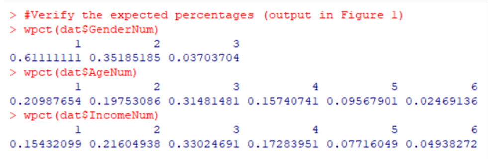
Figure 2: Observed percentages from the sample (consistent with Tables 1, 2, and 3).
Next, make sure the data columns in the data frame are defined as factors:
# Make sure data columns are factors
dat$GenderNum <- factor(dat$GenderNum, levels = 1:3,
labels = c(“Female”,”Male”,”Nonbinary”))
dat$AgeNum <- factor(dat$AgeNum, levels = 1:6,
labels = c(“18-24″,”25-29″,”30-39″,”40-49″,”50-59″,”60-69”))
dat$IncomeNum <- factor(dat$IncomeNum, levels = 1:6,
labels = c(“$0-$24k”,”$25k-$49k”,”$50k-$99k”,”$100k-$149k”,”$150k-$199k”,”$200k+”))
Then set the targets obtained from the reference population:
#Set targets
targets <- list(
GenderNum = c(Female = 0.505, Male = 0.485, Nonbinary = 0.010),
AgeNum = c(`18-24` = 0.128, `25-29` = 0.085, `30-39` = 0.171,
`40-49` = 0.155, `50-59` = 0.164, `60-69` = 0.297),
IncomeNum = c(`$0-$24k` = 0.19, `$25k-$49k` = 0.20, `$50k-$99k` = 0.30,
`$100k-$149k` = 0.15, `$150k-$199k` = 0.08, `$200k+` = 0.08)
)
The last step is to define case IDs for the data:
#Define case IDs starting from 1 to the length of any of the variables
dat$caseid <- 1:length(dat$GenderNum)
Now everything is ready to run anesrake and review a summary of its output (see Figure 3) and to print the weights for easy copying into the Excel file (see Figure 4)—targets, dat, and caseid are the required arguments for the anesrake function (for a full description of the required and optional arguments, see the anesrake specification):
#Calculate weights and print summary of results
outsave <- anesrake(targets, dat, caseid=dat$caseid)
summary(outsave)
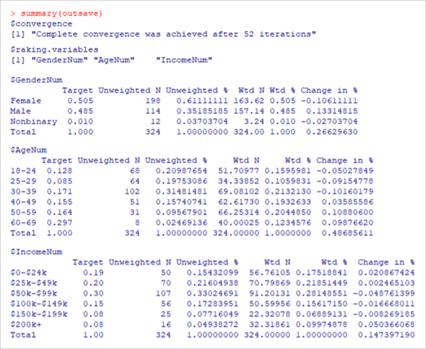
Figure 3: Key outputs of the anesrake summary showing the number of iterations to convergence (52) and the resulting weighted and unweighted counts and percentages.
# Print weights for each case to review
dat[“Weights”]
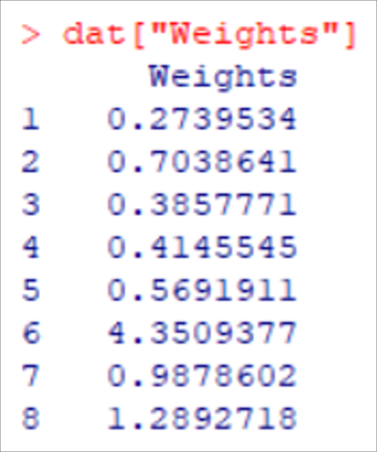
Figure 4: Weights for the first eight cases.
Finally, print the entire data frame to an Excel file to include the weights in the last column (Figure 5).
# Print data frame to Excel
write.xlsx(x = dat, file = “/Users/Jim/Documents/MeasuringU/Benchmarks/2024/Social Media/Social Media 2024 Rake Weights Exercise with Weights.xlsx”, sheetName = “Data”, colNames = TRUE, rowNames = FALSE, overwrite = TRUE)
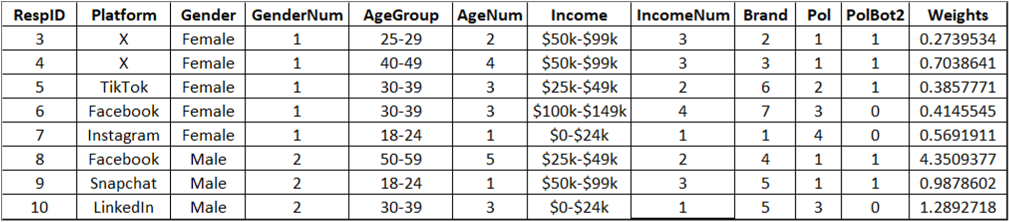
Figure 5: First eight rows of the printed Excel file with the rake weights.
The weights ranged from 0.119 to 5.0. The smallest weight was for the most overrepresented combination of demographic variables (nonbinary, 25–29, $150–$199k), and the largest was for the least represented (all respondents, 60–69 years old).
One aspect of the “art” of weighting is deciding whether to limit the range of weights to no less than 0.5 and no more than 2.0. As we’ve discussed in a previous article, this practice has some benefits (e.g., reducing the impact of weighting on the precision of group means), but it reduces the sum of the weights so they no longer match the sample size. For this reason, as in this example, we generally prefer to work with unadjusted weights.
Using Weights
The specific method for using weights depends on your statistical software. In the following examples, we’ve imported the data into SPSS and used its WEIGHT function (specifically, “WEIGHT BY Weights”) to get unweighted and weighted results for two questions from our social media survey.
Brand Attitude
Figure 6 shows the mean responses by platform for ratings of brand attitude on a seven-point scale (“Overall, how would you rate your attitude towards [social media platform]?”; 1 = Very Unfavorable; 7 = Very Favorable). The weighting slightly affected the mean ratings (by no more than 0.3 points for a given platform, 5% of the range of the scale) but did not change the interpretation of the results. Weighted or unweighted, TikTok had the highest brand attitude, X had the lowest, and the other platforms clustered together in the middle (slightly lower for Facebook).
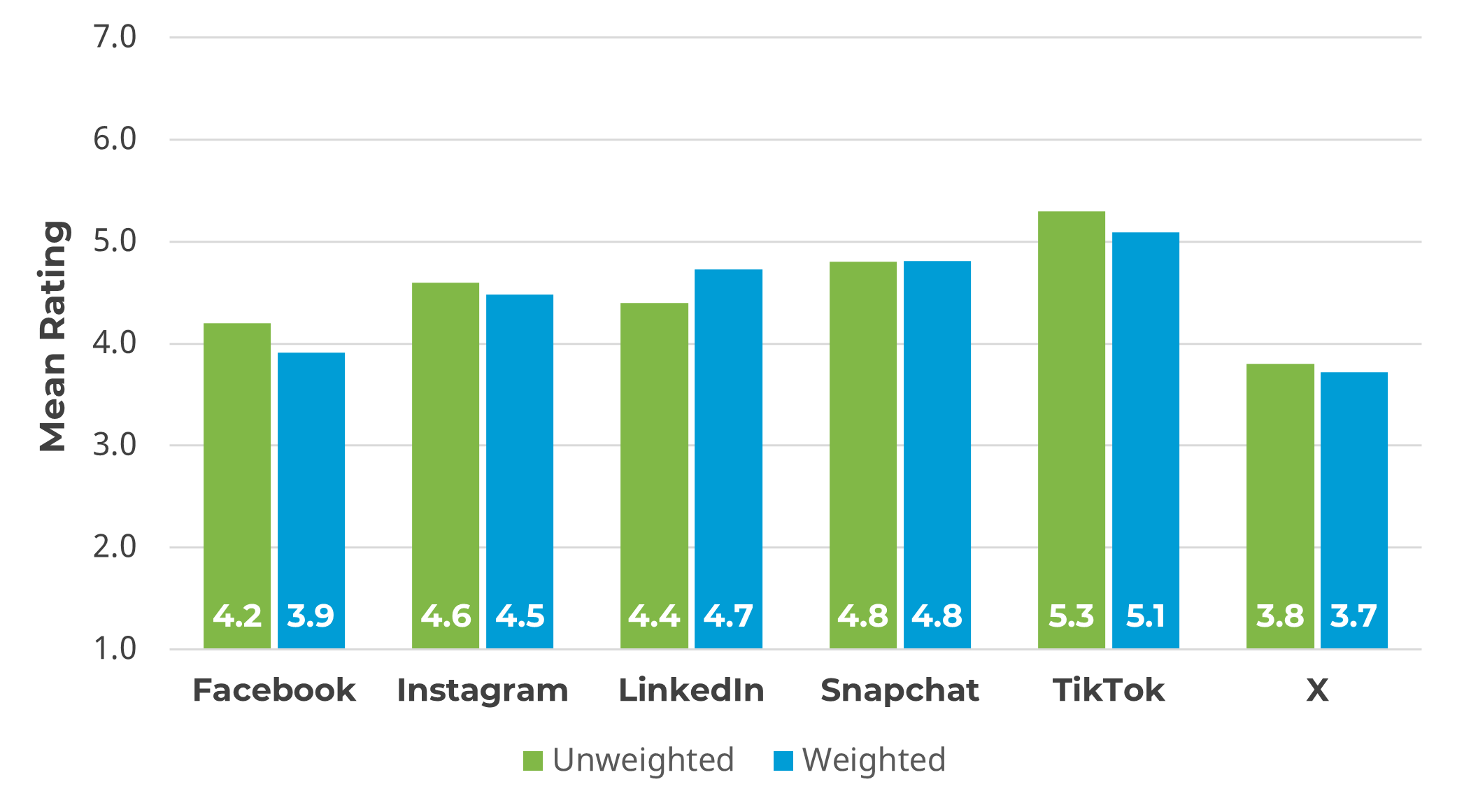
Figure 6: Mean ratings of brand attitude, unweighted and weighted.
Reluctance to Engage in Political Discourse
Respondents in the social media survey were asked “How likely are you to share political content on social media?” using a five-point scale from Very Unlikely (1) to Very Likely (5). Most respondents indicated a reluctance to engage in political discourse on their platforms, so one of our analyses of the results was as a bottom-two-box score, where larger percentages indicate greater reluctance to share political content (Figure 7).
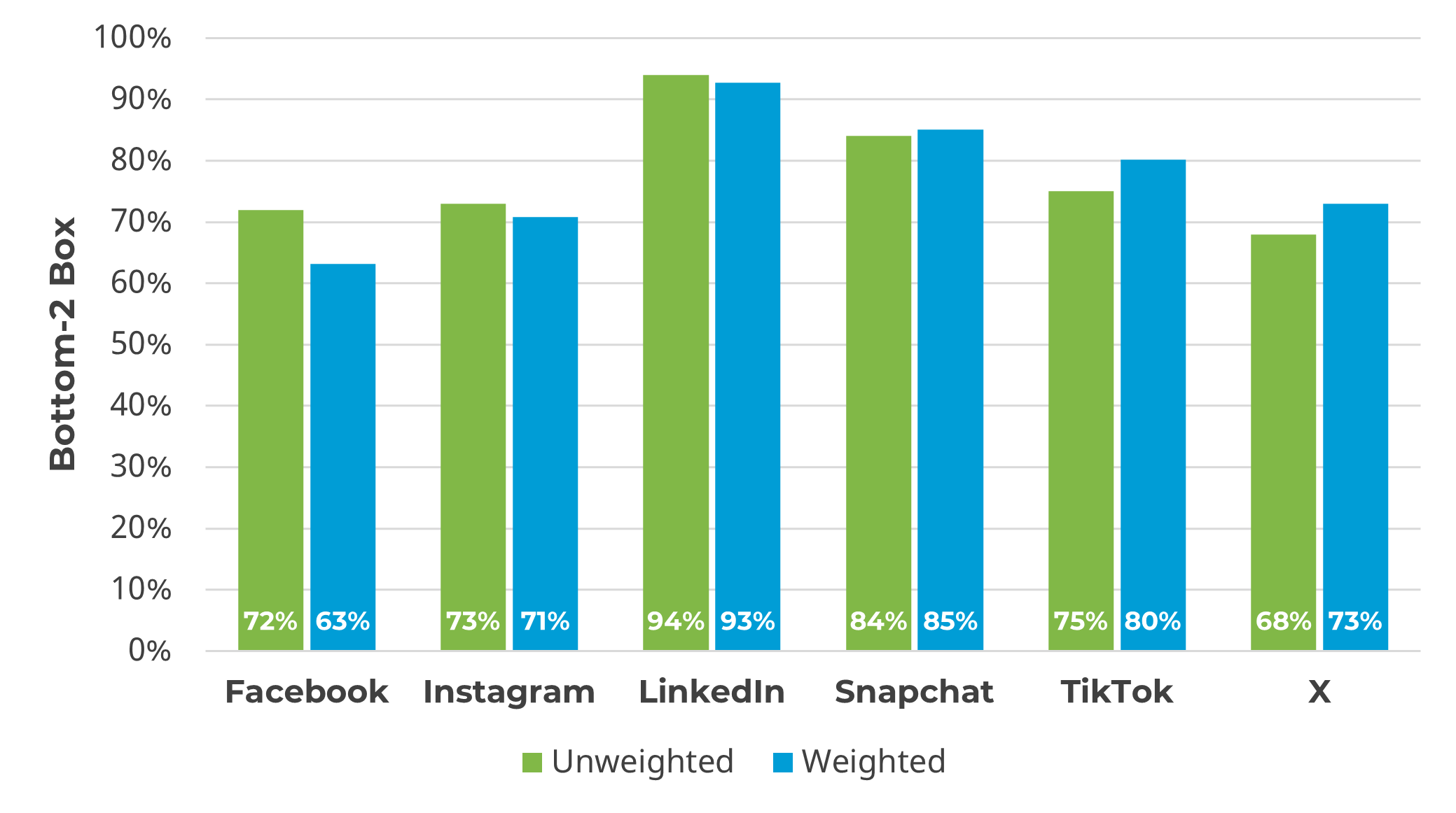
Figure 7: Bottom-two-box scores for likelihood of sharing political content, unweighted and weighted.
Like the first example, weighting had some effect on bottom-two-box percentages (the largest change was for Facebook from 72% to 63%), but little effect on the key narrative emerging from the data. With or without weighting, users of LinkedIn are especially reluctant to share political content. Although a majority of Facebook, Instagram, and X users selected a bottom-two response option, users of these platforms are more likely than LinkedIn users to share political content.
Summary and Discussion
When there is a need to weight multiple demographic variables to match a sample to a reference population, rake weighting is a popular option, and the R package anesrake is a popular tool. In this article, we discussed why and how to use rake weighting with a sample R script and examples applied to data from a 2024 survey of the UX of social media platforms. The key points in the article are:
Raking is rare in UX research but has its place. For some research questions, especially national voting estimates, weighting a sample to match the U.S. population is an important analytical step. Weighting is less common in UX research because there usually is no suitable reference population. For example, UX metrics are more affected by user characteristics such as the extent of experience with a product than by demographic variables such as gender, age, or income.
Rake weighting has significant advantages over other methods. Rake weighting is a popular approach to computing weights based on multiple participant variables because it requires input of only the sample and population for each variable (no need for complex crosstabs), and several open-source R packages perform rake weighting.
As expected, weighting with UX census data had little effect on the results from a UX survey of social media. To provide examples of rake weighting and its effect on UX analyses we conducted in 2024, we computed unweighted and weighted results for two items from a survey of the UX of social media platforms (mean ratings of brand attitude and bottom-two-box scores for likelihood to share political content on platforms). Weighting had very little effect on mean ratings of brand attitude. Weighting had slightly more effect on bottom-two-box percentages measuring the reluctance to engage in political discourse (the most political item in the survey) but still had no substantial effect on the interpretation of the results.
Bottom line: UX researchers should exercise caution in analyzing weighted rather than unweighted data unless there is a good reference population for the research questions. When there is a need to weight data based on multiple user characteristics, rake weighting is a popular and effective method.