“That design will never work.”

You may have had that thought before you even ran your first participant in a usability test.

If you’ve seen enough users struggle and conducted enough usability tests, then you probably have some idea about how well or poorly a task attempt may go for prototypes or even commercially available software or products.

It’s rare to have no idea about how well things will go before the testing even starts. In fact, an experienced researcher is expected to know of some problems and anticipate the friction. This is one of the foundations behind inspection methods like heuristic evaluation and the PURE method (which puts some numbers to friction).

Expert reviewers, of course, are not a substitute for observing users. But is there a way to build in our a priori knowledge of what’s likely to go wrong and then inform and update our beliefs once we see data? Can we do that systematically or even mathematically?

Thomas Bayes and Updating Our Beliefs from Data

It turns out that hundreds of years ago, a famous Presbyterian minister named Thomas Bayes was also interested in updating his beliefs with what he observed.

His name has been associated with a formula for updating our beliefs with data (Bayes’ Theorem). It follows a simple iterative process:

1. Start with a belief or hypothesis.
2. Collect data.
3. Update the belief.
4. Repeat.

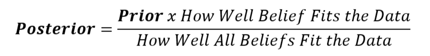
The formula for this process looks like this:

In other words, start with what you expect, check how well the data matches that expectation, and then adjust your belief accordingly.

The Bayes’ formula means that beliefs that better predict the data become more credible; beliefs that predict the data poorly lose credibility.

Our original belief is called the prior hypothesis (before). The belief we have after observing data and calculating an update is our posterior belief (after).

If we replace words with symbols, we get the more recognizable Bayesian formula. We have only two symbols that extend Bayesian thinking: θ (theta) and D (data).

Our prior belief is represented with the Greek symbol theta (θ) and shown in the formula as the probability of theta. D represents the data we observed/collected and is shown in the formula in the denominator (probability of all data). Both θ and D appear in the numerator as a conditional probability of the data given theta (D|θ).

Our posterior (updated belief) is represented with the probability of theta given the data (θ|D). The resulting formula is:

Interestingly, Bayes himself never published his famous theorem. It was published after his death by his friend Richard Price [PDF], who used it to attempt to prove the existence of God by showing that the order in the universe wasn’t accidental. Because Price likely made a substantial contribution to completing Bayes’ work on the theorem, this may be another example of Stigler’s Law (scientific discoveries are not named after the discoverer or, in this case, do not include the co-discoverer).

Formulas, ministers, and theology are interesting and all, but how does this apply to UX research?

A Simple UX Research Example with Completion Rates

We can use an example of testing a new checkout experience. We want to gauge the completion rate (a fundamental usability metric). How successfully are people able to get through the new flow?

We’ve never tested this checkout flow before, though. But do we really have no idea about what will happen? Is a 0% completion rate really as likely as a 50%, 90%, or 100% completion rate?

Using a rough guide from historical data, we know an “average” completion rate is around 78%. It doesn’t mean we expect this new checkout completion rate to be exactly 78% (there is a lot of variability around this average). But values between 50% and 95% seem more plausible than a 5%, 10%, or even 99% completion rate. The lower end would be cause for concern, and the upper end would be desired for such an important flow.

What Exactly Is Our Prior?

So, following Bayesian thinking, we establish a prior. Our prior belief is not a single number (78%), but a range of plausible completion rates, centered near 78% (the most plausible rate). Rates far lower (e.g., 40%) or far higher (e.g., 99%) are possible but less likely. In Bayesian terms, this represents a prior belief with a probability distribution centered at 78% but wide enough to allow for substantial uncertainty (see the appendix for details).

Collecting Data

As an example of using data to update our initial thinking, assume we’ve collected data from a hypothetical moderated usability test with twenty participants in which eighteen completed the checkout and two failed. That’s a 90% observed completion rate. What does that do to our prior belief?

Using Bayesian thinking, we’d ask which completion rates best explain 18 successes out of 20.

• Rates near 90% explain it well.
• Rates near 78% still explain it reasonably well.
• Rates near 50% explain it poorly.

Bayes’ theorem formalizes that comparison. It increases the credibility of rates that better predict the data and decreases the credibility of those that don’t.

Updating Our Prior

Before seeing the data, our belief was centered near 78%. After observing 18/20 completions, we conclude (see appendix for the mechanics):

• Our updated best estimate of the true completion rate is about 86%.
• A 95% credible interval runs from roughly 72% to 96%.
• There’s about an 89% probability that the true completion rate exceeds 78%.

A few things to notice:

• The data pulled our estimate up from 78% toward 90%.
• It didn’t go all the way to 90%.
• The prior kept us from overreacting to just twenty observations.

That’s Bayesian updating. We started with an informed expectation, saw new evidence, and adjusted accordingly. Figure 1 illustrates this Bayesian thinking.

Figure 1: The posterior distribution (after observing 18/20 completions) shifts upward from the prior centered at 78%, reflecting the influence of new data while retaining uncertainty.

So, can we just plug our numbers into the simple formula we showed above? The answer we’ve found working through this Bayesian example is, unfortunately, not that simple. We describe the approach we used for those numbers below in the appendix.

We’ll cover how to conduct these analyses in upcoming articles, but this provides some idea about using Bayesian thinking in practice without getting swallowed up in the conditional probabilities.

Updating Our Beliefs with More Questions

Who can argue with updating your beliefs with new data? We like this idea of applying iterative Bayesian thinking and incorporating historical data. Who wants to be stuck in their ways? But while using Bayesian thinking seems both appealing and like sound science, it generates a few questions:

• How is this different from using the statistics taught in an intro statistics class and our courses?
• What’s the difference between a credibility interval and a confidence interval?
• Do Bayesian statistics require smaller sample sizes?
• What if you don’t have any prior information?
• How reliable are priors if they are just our intuition or “conventional wisdom?”
• Can a prior steer us in the wrong direction?
• How can this concept be extended to assessing the likelihoods of different hypotheses?

We’ll dig into these questions in upcoming articles.

Appendix: How the Posterior Was Computed

Here’s a quick summary of how we computed the values. We used some common modern Bayesian methods that are computationally intense (we’ll cover that in a future article).

We modeled the true completion rate using a Beta distribution and the observed data using a binomial model. We set a weak prior centered at the historical average of 78%, equivalent to about 10 prior observations. This corresponds to a Beta(7.8, 2.2) prior distribution.

With 18 completions out of 20 participants, the Bayesian update is: for a Beta prior and binomial data, the posterior is Beta(α + successes, β + failures). Substituting the values gives a posterior of Beta(25.8, 4.2).

From this updated distribution:

• The posterior mean is 25.8/30 ≈ 86%.
• The 95% credible interval is approximately 72% to 96% (2.5^th and 97.5^th percentiles of the Beta(25.8, 4.2) distribution.
• The probability that the true completion rate exceeds 78% is about 89% (using the upper tail of the Beta(25.8, 4.2) distribution.

This update reflects a compromise between prior expectations and observed data, with the new evidence pulling the estimate upward while retaining uncertainty.