 Paraphrasing the statistician George Box, all models are wrong, some are useful, and some can be improved.
In a recent article, we reviewed the most common way of modeling problem discovery, which is based on a straightforward application of the cumulative binomial probability formula: P(x≥1) = 1 – (1-p)n.
Well, it’s straightforward if you like playing around with these sorts of formulas like Jim and I do.
In this formula, p is the probability of an event of interest (e.g., a participant experiences a specific usability problem), n is the number of opportunities for the event to occur (sample size), and P(x≥1) is the probability of the event occurring at least once in n tries. In other words, if you know n and p, you can estimate the likelihood of discovering (seeing at least once) a usability problem.
For the formula to work, you need a value for p. In the most common method, p is estimated from a participant-by-problem matrix. When the sample size is large, binomial models using estimates of p tend to closely match empirical problem discovery. When the sample size is small, however, estimates of p tend to be inflated and lack correspondence with empirical problem discovery, so the projected rate of problem discovery would be faster than it actually is.
Another potential issue with estimates of p aggregated across a set of problems with different likelihoods of occurrence is that the binomial probability model doesn’t have any parameters that account for the variability of p. This can lead to a phenomenon known as overdispersion, where the problem discovery model is overly optimistic compared to empirical problem discovery.
Despite these issues, this original approach to modeling problem discovery is usually accurate enough to be useful. In this article, we explore some approaches to improving this wrong but useful model.
Binomial p (Adjusted)
Before 2001, a common practice was to run a test with a few participants and then use those results to estimate p. With that estimate, you could use the cumulative binomial probability equation to predict how many participants you would need to achieve a specific percentage of discovery (acknowledging the generalizability limits due to product, tasks, participants, environments, and methods). Based on the pilot data, you could also predict for each sample size how many unique usability problems you would probably discover and how many would probably remain undiscovered. A flaw in this procedure was revealed by Hertzum and Jacobsen (2001*), who demonstrated that this would always overestimate the true value of p, where “true” is the value of p at the end of a large-sample study. (* This paper first appeared in 2001, but due to printing issues for some figures, was republished in 2003.)
Recalling the example from our previous article, Virzi (1990) published a participant-by-problem matrix with data showing the discovery of 40 problems in a study with 20 participants. When we estimated p from a randomly selected set of three participants, we got .59—a substantial overestimate of the value of p generated from the full study (.36). With n = 3 and p = .59, the expected percentage of discovery from the cumulative binomial probability is .93 (93%). There were 25 problems detected with those three participants, so the estimated number of problems available for discovery using that value of p is 27 (25/.93), far fewer than the 40 problems reported by Virzi.
Inspired by Hertzum and Jacobsen, Lewis (2001) developed a systematic method for reducing small-sample estimates of p using the following equation (see the article for its derivation):
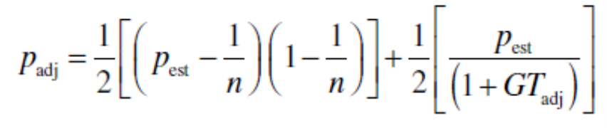
Figure 1: Formula for adjusting observed estimate of p (Lewis, 2001).
The adjusted value of p is the average of two independent ways to reduce its value. The first is driven by the sample size, and the second is an application of Good-Turing discounting based on the number of problems that were observed just once in the sample.
If we use the formula in Figure 1 to adjust that initial estimate of p (.59), we note that the first three participants found 11 of the problems only once. With this information, the first method, which tends to bring the value of p down too much, gets p = .17. The second method, which tends to leave p too high, gets p = .41. The average of the two is the adjusted value of p is .29.
When using this adjusted estimate of p, the predicted amount of discovery when n = 3 is .64, so the estimated number of problems available for discovery is 39 (25/.64), very close to the observed number of 40.
Binomial p (Targeted)
Despite their general success in modeling problem discovery, methods based on estimates of binomial p, adjusted or not, can be criticized because they don’t account for the variability in point estimates aggregated across problems of varying probability of occurrence. One way to avoid this issue is to pick a target value of p instead of estimating it (Lewis, 2012). Table 1 shows likelihoods of discovery for various targets of p and sample sizes, computed using the cumulative binomial probability formula.
| p | n = 5 | n = 10 | n = 15 | n = 20 |
|---|---|---|---|---|
| 0.01 | 0.05 | 0.10 | 0.14 | 0.18 |
| 0.05 | 0.23 | 0.40 | 0.54 | 0.64 |
| 0.1 | 0.41 | 0.65 | 0.79 | 0.88 |
| 0.25 | 0.76 | 0.94 | 0.99 | 1.00 |
| 0.315 | 0.85 | 0.98 | 1.00 | 1.00 |
| 0.5 | 0.97 | 1.00 | 1.00 | 1.00 |
| 0.75 | 1.00 | 1.00 | 1.00 | 1.00 |
| 0.9 | 1.00 | 1.00 | 1.00 | 1.00 |
Table 1: Discovery likelihood for various targets of p.
For example, suppose you want to have a pretty good (>90%) chance of discovering problems that are likely to occur 25% of the time (within the constraints of your study, as described above). Table 1 shows that you probably won’t achieve this goal with n = 5, but you probably will with n = 10. For another example, suppose you want to discover 80% of the problems that will happen 5% of the time. Table 1 shows that you won’t be likely to achieve this goal even when n = 20, so you’d either need to plan for a larger sample size (n = 31) or set a different target for p. We use this approach at MeasuringU when scoping projects with clients, balancing sample sizes and budgets/timelines for testing.
Beta-Binomial and Other Complex Models
Another way to deal with the issue of binomial variability is to use beta-binomial modeling, which is designed to deal with the overdispersion in binomial modeling that can lead to overly optimistic estimates of problem discovery. Schmettow (2008) reported comparisons of adjusted-p and beta-binomial modeling of five problem discovery databases in which the beta-binomial model was a better fit in three cases and adjusted-p modeling was better in two cases. Other more complex approaches that can be used to modeling problem discovery include
Because the less complex models work reasonably well in practice, we have not yet investigated any of these more complex models, but we are interested and plan to study them in the future.
When Problem Discovery Gets Foamy
There has been some success with having an idea about the general number of problems to uncover, especially when the problems are common. But one of the shortcomings we’ve noticed is that these models tend to underpredict the observed number of problems, especially when the sample sizes get large, even when the interface, tasks, and participant profile don’t change.
The more users tested, it seems, the more problems are uncovered. It’s unusual to see a common problem emerge after having tested earlier with several participants. Instead, what’s seen are a lot of uncommon, idiosyncratic issues experienced by one or a few participants.
For example, Figure 2 uses data from Lewis (2001; MACERR data available in the appendix) to show how discovery of 145 unique problems tailed off as additional participants (n = 15) completed a set of office automation tasks. The first participant uncovered 38 problems. Of the 145 unique problems, 76 occurred only once, constituting the “problem foam.” Each of the 15 participants encountered these idiosyncratic problems. Even though the unadjusted, overall estimate of p for this matrix was just .16, the figure shows that most (but, as expected, not all) of the most frequently occurring problems were discovered within the first five participants. After the fifth participant, only three problems were experienced by more than two participants.
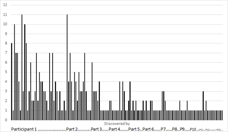
Figure 2: Number of occurrences of each of the 145 unique usability problems across 15 participants.
It’s almost as if there are two classes of usability problems, not necessarily with a clear division. One class contains problems that behave as predicted by problem discovery models. The other class of problems is foamy, with bubbles (problems) popping up chaotically, analogous with the emergence of matter at the edge of black holes due to quantum foam. Or, using a less cosmic analogy, compare Figure 2 with Figure 3, which shows an audio signal recorded in the presence of static.

Figure 3: Audio signal with background static.
One possible explanation for new problems emerging even after testing many users is that the individual differences each participant brings (prior experiences, assumptions, different mental models) increases the chances for unique interactions and, consequently, additional unique problems.
Note that UX practitioners who conduct usability studies shouldn’t ignore problems that happen only once. You have to wade into the foam/static. Frequency of occurrence is only one property of a usability problem. Severity (impact) is not correlated with frequency, so it’s always possible that a usability study might uncover infrequent but high impact problems that need to be addressed in future design iterations.
A New Model: Cubic Regression
We’re always interested in new approaches to modeling problem discovery. Somewhat recently (in 2013), Bernard Rummel noticed a pattern with his usability problem datasets, which he shared with us. As shown in Figure 4, he found that the cumulative number of unique problems detected could be modeled as a cubic function relative to the sample size.
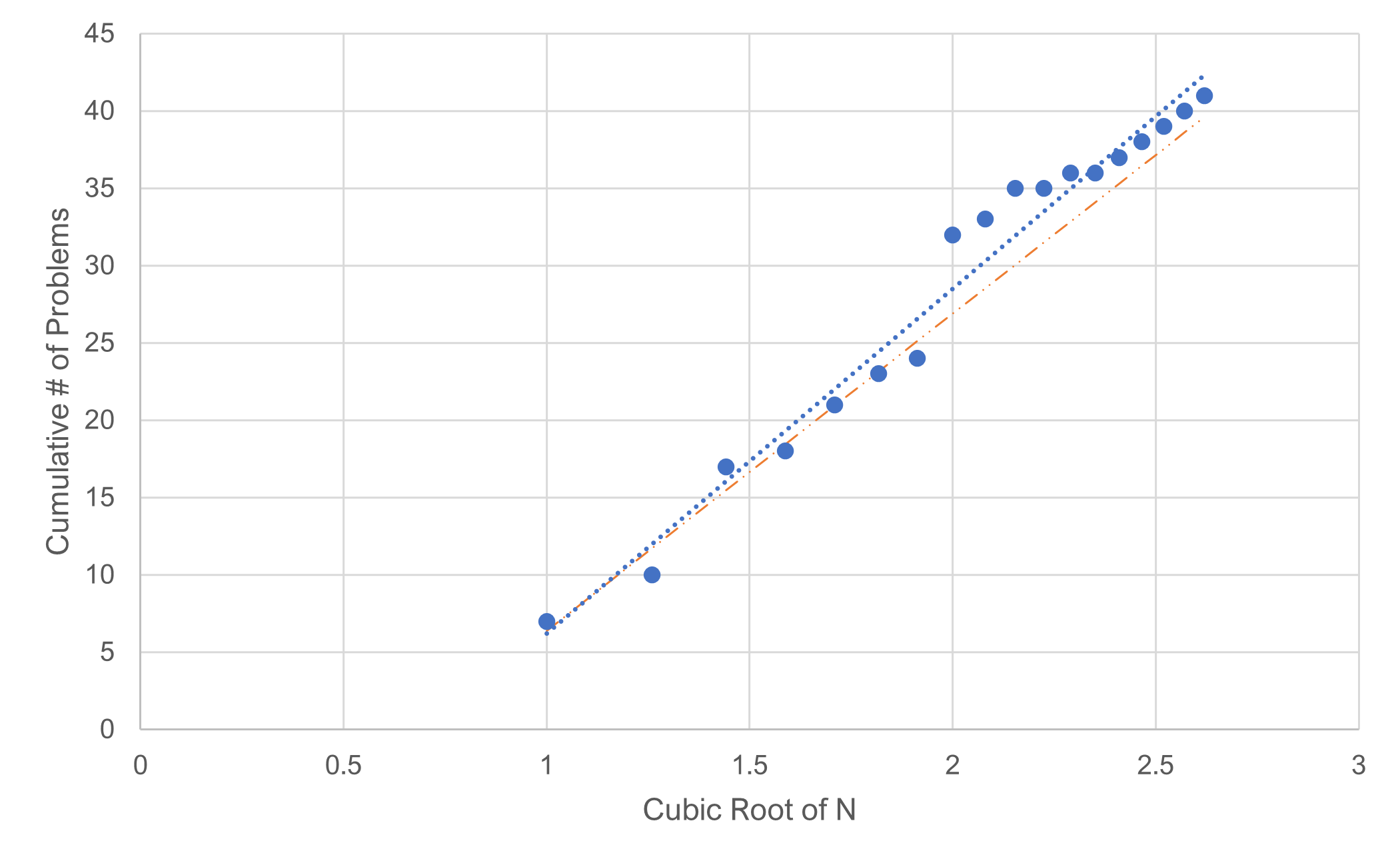
Figure 4: Modeling the cumulative number of problems with an N-cubic function (data comes from a usability test with 18 users and 38 unique problems uncovered).
The Y-axis shows the total number of unique problems uncovered in one usability study with a sample size of 18 and 38 unique problems found. The X-axis is the cube root of the sample size. You’re probably familiar with the square root, which is the number you multiply by itself twice to get the original number. For example, the square root of 9 is 3 (3×3). The cube root is the same number multiplied by itself three times. So, the cube root of 8 is 2 (2x2x2).
What this approach suggests is that an interface has an unlimited number of problems. These problems become vanishingly sparse as your sample size grows unrealistically large, but you will continue seeing new problems as you test users.
Similar to the adjusted-p approach, this model uses the first five data points to build an equation for a line [regression equation (intercept and slope)]. Was this one data set a fluke, or is there a consistent pattern where we can model using a cubic relationship? We’ll explore this model in depth and compare it to the other models in an upcoming article.
Summary and Takeaways
The most common approach to modeling problem discovery is to estimate the overall likelihood of problem occurrence (p) and use that in the cumulative binomial probability formula.
This common approach can be useful, but it’s problematic in two ways. First, estimates of p made from small-sample usability studies are necessarily overestimated. Second, any method that estimates an overall value of p across problems with different likelihoods of occurrence is open to criticism for not taking variability of p into account in the model.
One way to address these criticisms is to set a target value for p instead of estimating it. Another way is to model problem discovery with more complex models such as beta-binomial or capture-recapture.
Another potential criticism of models that predict the likely percentage of discovery is based on the observation that even though discovery slows down as you observe more participants, it never seems to stop completely. Once the frequent problems are discovered, there is still a residue of problem “foam” or “static.”
A new approach to modeling the cumulative number of unique problems, based on the cube root of the sample size, has shown promise and doesn’t explicitly assume a finite number of problems available for discovery. We plan to look into this method and will explore it in an upcoming article.