 Finding and fixing problems in an interface is one of the fundamental priorities of a formative usability test.
But how many users should you test with? And how many usability problems are there to be uncovered? These questions have been discussed and debated for decades.
Early work on problem discovery suggested that the first few users will uncover most of the common problems. This isn’t—or shouldn’t be—controversial: The first participants (say the first 1–5 or so) will find most of the most common problems. It’s a mathematical truism, and it’s something we’ve confirmed empirically with our own data. In our analysis of seven usability problem sets, we found that the first five users uncovered 91% of the most common issues (affecting, on average, 54% of users).
Where things get less certain—and more controversial—is when we want to estimate more precisely how many users we need to test. The more users, the more problems you will uncover, and the fewer problems left undetected, but as is the case in many usability studies, recruiting more users is time- and cost-prohibitive. Finding the right sample size is then a function of how common the problems are and how many of the problems you hope to detect. So, how can we predict the number of problems? We use models.
Predicting the Percentage and Number of Problems Detected and Undetected
All models are wrong. Some are useful.
The statistician George Box is credited with that statement, and no doubt you’ve experienced incorrect predictions made from models, including projections on presidential victories, COVID hospitalizations, and whether it will rain tomorrow.
There have been several published approaches to modeling problem discovery. Most methods require estimates of the average likelihood of problem occurrence which, as described below, can be problematic. These models are based on the binomial distribution of the problem occurrence (p), an adjusted problem occurrence, the beta-binomial, more complex models, and a new entrant based on the cubic root of the sample size. We’ll cover the average problem occurrence method in this article and the others in an upcoming one.
Binomial p (estimated)
The earliest (and still most common) approach is to use the cumulative binomial probability formula. We show the derivation of the following equation in Quantifying the User Experience.
P(x≥1) = 1 – (1-p)n
In this formula, p is the probability of an event of interest (e.g., participant experiences a specific usability problem), n is the number of opportunities for the event to occur (sample size), and P(x≥1) is the probability of the event occurring at least once in n tries. In other words, if you know n and p, you can estimate the likelihood of discovering (seeing at least once) a usability problem with probability p. (Just to confuse you, some published versions of the formula use the Greek Lambda (λ) instead of p.)
This equation was used to justify the “Magic Number 5.” In a 1993 literature review of usability studies, Nielsen and Landauer found the average value of p across several studies to be .31.
If you put .315 in the equation for p and 5 for n, you get .85 (85%). Over time, some mistakenly interpreted this result as “All you need to do is watch five people and you’ll find 85% of a product’s usability problems.” A better interpretation is “If you watch five users, you should discover about 85% of the problems that will happen to 3/10 of all users of the interface.” You will also find a smaller percentage of less likely problems and a larger percentage of more likely problems.
This is true as long as the constraints of the study hold: same tasks, same sample characteristics, same test environment, and same test method. With those constraints in mind, this model works pretty well for given sets of data. For example, Figure 1 shows the results of binomial estimation with the data from Virzi (1990), one of the first papers to publish the kind of participant-by-problem matrix needed to model this kind of discovery (Table 1).
To estimate p from the full matrix shown in Table 1, you take the average of all the 0s and 1s, which is .36. The graph in Figure 1 shows the discovery percentage predicted with p = .36 for each sample size from 1 through 20. It also shows the empirical discovery curve obtained with Monte Carlo randomization of the order of participants for comparison with the predicted curve. The curves aren’t exactly the same, but they’re close (identical at the beginning and end).
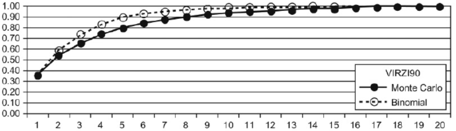
Figure 1: Demonstration of close correspondence between binomial discovery model and empirical Monte Carlo distribution for data from Virzi (1990).
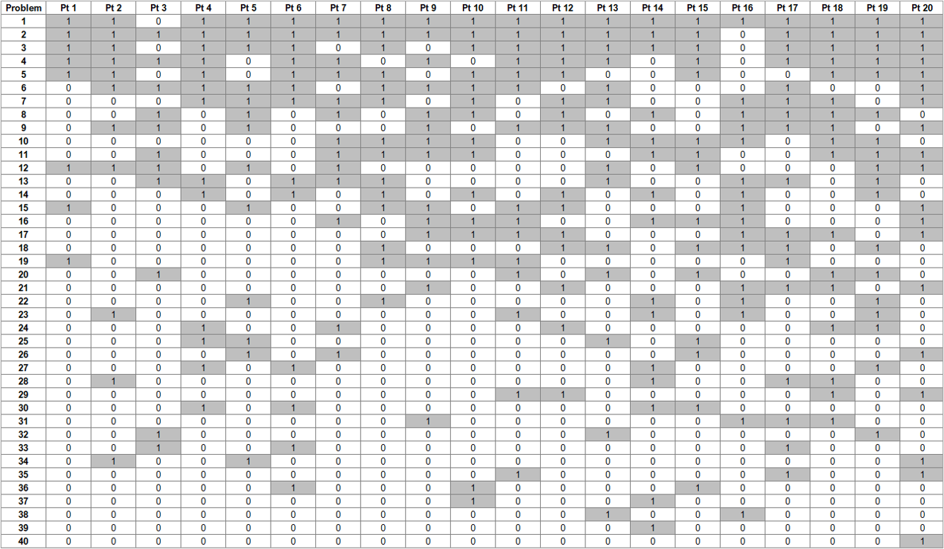
Table 1: Participant-by-problem matrix from Virzi (1990), with problems arranged from easiest to most difficult to discover and participants arranged from least to most problems encountered.
Problems with p
Although models and graphs based on estimates of p have been useful in UX research, they have limitations, especially when planning usability studies. To use them in planning, you need to have an estimate of the overall rate of problem discovery—p in the equation—and the current literature has reports from large-sample studies of p ranging from .03 to .60. After you’ve run a study and obtained a full participant-by-problem matrix with a reasonable sample size, you’ve got a pretty good estimate, but by then the study is over.
Before 2001, a common practice was to run a few participants, say two to five, and then use those results to estimate p. With that estimate, you could use the cumulative binomial probability equation to estimate how many participants you would need to run to achieve a specific percentage of discovery (acknowledging the generalizability limits due to product, tasks, participants, environments, and methods). Based on the pilot data, you could also predict for each sample size how many unique usability problems you would probably discover and how many would probably remain undiscovered.
In 2001*, however, Hertzum and Jacobsen demonstrated that this method of estimating p would always overestimate its value because the initial participant-by-problem matrix can’t contain information about problems that haven’t been discovered yet. (* Their paper first appeared in 2001, but due to problems in journal production of some figures, was republished in 2003.)
To illustrate this, we randomly selected three participants (8, 11, and 12) from Table 1. When you estimate p using all 40 unique problems from Table 1, p = .37, which is close to the estimate with the full matrix. However, for those three participants, there are 15 problems that they did not encounter. When you remove those problems from the partial matrix and recalculate p using the information available with just those three participants, you get .59, a substantial overestimate.
Table 2 shows the impact of this example’s overestimation. Assuming p = .59, you would think you have a discovery rate of about 83% by the second participant, but assuming p = .37, you wouldn’t expect that until the fourth participant. There were 25 problems detected with those three participants, so assuming p = .37, the estimated number of problems available for discovery is about 33 (25/.75), but assuming p = .59, that estimate would be just 27 (25/.93). Both values underestimate the actual number of 40 unique problems discovered in the study.
| n | p = .37 | p = .59 |
|---|---|---|
| 1 | 0.37 | 0.59 |
| 2 | 0.60 | 0.83 |
| 3 | 0.75 | 0.93 |
| 4 | 0.84 | 0.97 |
| 5 | 0.90 | 0.99 |
| 6 | 0.94 | 1.00 |
| 7 | 0.96 | 1.00 |
| 8 | 0.98 | 1.00 |
| 9 | 0.98 | 1.00 |
| 10 | 0.99 | 1.00 |
Table 2: Expected discovery when p = .37 and when p = .59.
So is this model too wrong to be useful? In a future article, we’ll summarize other methods that are currently under investigation to improve predictions of the number of unique problems likely to occur in formative usability studies.
Summary and Takeaways
A key step in determining the appropriate sample size for a formative (problem discovery) usability study is estimating problem frequency (p).
Early research in modeling problem discovery relied on estimates of p obtained from large-sample usability studies and plugged into the cumulative binomial probability formula to predict the likely percentage of discovery as a function of sample size.
The formula is useful in some ways but limited in how it can inform sample size estimation based on small-sample usability pilot studies. These problems have led to the development of methods to improve small-sample estimates of problem discovery, which will be the topic of a future article.


