

 The large sample size. The right statistical tests. A compelling and statistically significant finding! All the ingredients of a successful quantitative project that gets stakeholder buy-in. But inflation isn’t just a worry for the Federal Reserve on interest rate policy. It affects research decisions, too.
When you conduct something like a usage and attitude survey with hundreds or thousands of participants (like what we do with our industry reports), you have the benefit of statistical power (the ability to detect differences). This allows you to look not only for differences between main effects (like between software products), but also for interactions (differences by type of user by product).
With enough power, you can dig into these more nuanced differences. For example, you may learn that younger adults have different usage patterns and attitudes than older cohorts for certain products. It would be a compelling story, and it’s something that stakeholders can make sense of and act on. We’ve seen it and reported it. But how do you know these differences aren’t a fluke?
You may think limiting yourself to reporting only statistically significant findings will protect you from these false positives, and that approach certainly helps. But like printing money to boost the economy, the more statistical tests you run, the more you inflate your chances of finding things that aren’t actually there.
This isn’t monetary policy; it’s alpha inflation. It’s a subtle concept that you should understand when making multiple statistical comparisons.
Alpha (False Alarm Rate) in Hypothesis Testing
In null hypothesis significance testing (NHST), the alpha criterion is the value selected for decisions of statistical significance. This is the process through which you decide if a difference is statistically significant. As shown in Figure 1, when the p-value you get from a statistical test is less than the alpha value you set, you reject the hypothesis of no difference (the null hypothesis, H0). It’s statistical significance! Otherwise, you fail to reject H0 (you don’t accept it; you just don’t have enough evidence to reject it).
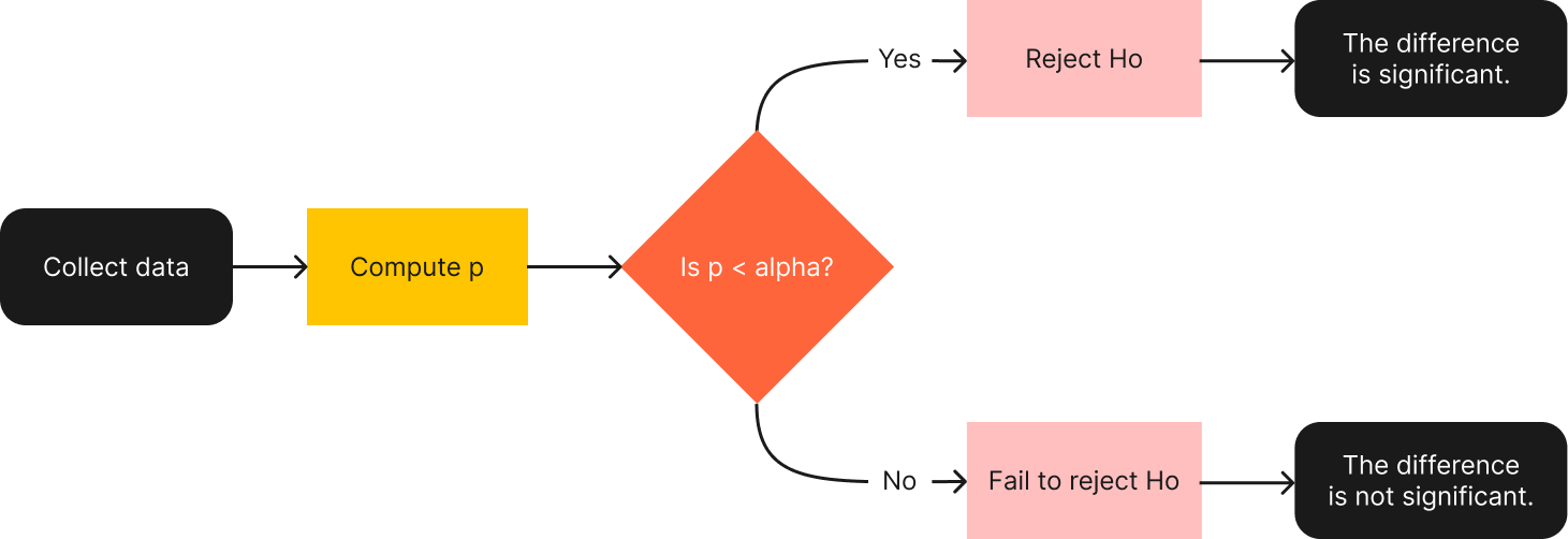
Figure 1: High-level flowchart of statistical hypothesis testing.
The whole point of this process is to control the percentage of false alarms (rejecting H0 when there really is no difference) in the long run. We’ve previously discussed why the alpha criterion doesn’t have to be the standard p < .05, but the rationale for using .05 was published by R. A. Fisher in 1929: “It is a common practice to judge a result significant, if it is of such a magnitude that it would have been produced by chance not more frequently than once in twenty trials [.05]. This is an arbitrary, but convenient, level of significance for the practical investigator.”
So, when you run one test of significance, if there is really no difference, you have a 5% chance of mistakenly concluding that there is a difference. That’s fine if you’ve collected data from two groups (A and B), but what if you’ve collected data from three groups (A, B, and C) and want to compare A with B, B with C, and A with C? Or, as in the case of the usage and attitude survey, you want to make dozens of comparisons of subgroups (such as age or usage levels across product versions)?
For all these scenarios, you’ll have to deal with the consequences of alpha inflation.
What Is Alpha Inflation?
When we declare a difference as statistically significant when p < .05, we reduce our chance of being fooled by random noise in our sample. But these false alarms, called Type I errors in statistical jargon, will happen and are expected.
At the p < .05 level of significance, 5% of our conclusions will be false alarms over the long run. That’s 5% for running just one statistical test (such as comparing the UX-Lite® scores of two products). But what if you run more than one statistical test? Software makes it very easy to run all sorts of comparisons such as the differences between age cohorts, experience levels, and products. What if you run 5, 10, 20, or 100 tests? You’re printing money and, like the inflation rate, your false alarm rate goes up too.
To understand how running more tests increases your false alarm (Type I) error rate, Table 1 shows the probability of zero false alarms, one false alarm, two false alarms, and so forth.
| x (Number of false alarms) | p(x) when α = .05 | p(at least x) when α = .05 |
|---|---|---|
| 0 | 0.36 | 1.00 |
| 1 | 0.38 | 0.64 |
| 2 | 0.19 | 0.26 |
| 3 | 0.06 | 0.08 |
| 4 | 0.01 | 0.02 |
| 5 | 0.002 | 0.003 |
| 6 | 0.0003 | 0.0003 |
| 7 | 0.00003 | 0.00003 |
| 8–20 | 0.00000 | 0.00000 |
Table 1: Alpha inflation for 20 tests conducted with α = .05.
As shown in Table 1, the most likely number of Type I errors in a set of 20 independent tests with α = 0.05 is one, with a point probability of 0.38. That is, when you run 20 comparisons, there’s a 38% chance of getting one false alarm. The next highest point probability is 0.36 for 0 false alarms, meaning you have about the same chance of having no false alarms in a set of 20 comparisons as you do one false alarm.
Unfortunately, you can encounter more than one false alarm in a set of 20 tests. The likelihood of at least one Type I error, however, is higher (specifically, 1 − p(0) = 1 − 0.36 = 0.64). That’s a 64% chance of 1, 2, 3, or more. (Although more than two or three false alarms in 20 comparisons is rare.) So, rather than having a 5% chance of encountering a Type I error when there is no real difference, α has inflated to 64%.
What Can You Do About Alpha Inflation?
You can’t raise interest rates to tame alpha inflation. But since the middle of the 20th century, many strategies and techniques have been published to guide the analysis of multiple comparisons, such as omnibus tests (e.g., ANOVA and MANOVA) and procedures for the comparison of pairs of means (e.g., Tukey’s WSD and HSD procedures, the Student–Newman–Keuls test, Dunnett’s test, the Duncan procedure, the Scheffé procedure, the Bonferroni adjustment, and the Benjamini–Hochberg adjustment).
With all these methods available to handle alpha inflation, the problem is solved—right?
Controlling Alpha Inflation Has Its Consequences
When the null hypothesis is not true, applying techniques to control alpha inflation (decreasing the number of Type I errors) necessarily increases the number of Type II errors—the failure to detect differences that are real. An overemphasis on the prevention of Type I errors leads to the proliferation of Type II errors.
Unless, for your situation, the cost of a Type I error is much greater than the cost of a Type II error, you should avoid applying any of the techniques designed to suppress alpha inflation. As Perneger (1998, p. 1236) wrote, “Simply describing what tests of significance have been performed, and why, is generally the best way of dealing with multiple comparisons.” In UX and many applied research settings, failing to detect a real difference can be just as harmful as falsely declaring a difference. Context matters, so don’t think Type I errors should take all the focus.
Or, as Abelson (1995, p. 70) put it, “Random patterns will seem to contain something systematic when scrutinized in many particular ways. If you look at enough boulders, there is bound to be one that looks like a sculpted human face. Knowing this, if you apply extremely strict criteria for what is to be recognized as an intentionally carved face, you might miss the whole show on Easter Island.”
We pay more attention to alpha inflation when we’re making many unplanned comparisons. But even then, we have a balanced approach to managing Type I and Type II errors, which we’ll cover in an upcoming article.
Summary and Discussion
Alpha inflation is what happens when running multiple statistical tests quietly erodes the reliability of your p < .05 threshold, the same way printing money erodes the value of a dollar. The main points from this article are:
Alpha inflation is real. Run 20 independent comparisons at α = .05, and you don’t have a 5% chance of a false alarm anymore; you have a 64% chance of at least one. The reality of alpha inflation can easily be demonstrated using binomial probabilities (as in Table 1).
Many methods have been developed to control alpha inflation. The methods, primarily developed in the 20th century, vary considerably in their relative conservatism (judging fewer contrasts to be significant) and liberalism (judging more contrasts to be significant).
But you can’t just raise interest rates to fix alpha inflation. Controlling alpha inflation has hidden costs. Controlling only Type I errors (false alarms) leads to a proliferation of Type II errors (misses). The decision to use methods to control alpha inflation depends strongly on the relative costs of Type I and Type II errors in a specific research context. We’ll cover how to strike that balance in an upcoming article.