Making decisions with data inevitably means working with statistics and one of its most common frameworks: Null Hypothesis Significance Testing (NHST).
Hypothesis testing can be confusing (and controversial), so in an earlier article we introduced the core framework of statistical hypothesis testing in four steps:
- Define the null hypothesis (H0). This is the hypothesis that there is no difference.
- Collect data. Compute the difference you want to evaluate.
- Compute the p-value. Use an appropriate test of significance to obtain the p-value—the probability of getting a difference this large or larger if there is no difference.
- Determine statistical significance. If the value of p is lower than the criterion you’re using to determine significance (i.e., the alpha criterion, usually set to .05 or .10), reject the null hypothesis and declare a statistically significant result; otherwise, the outcome is ambiguous, so you fail to reject H0.
But just because you’re using the hypothesis testing framework doesn’t mean you will always be right. The bad news is that you can go through all the pain of learning and applying this statistical framework and still make the wrong decision. The power in this approach isn’t in guaranteeing always being right (that’s not achievable), but in knowing the likelihood that you’re right while reducing the chance you’re wrong over the long run.
But what can go wrong? Fortunately, there are only two core errors, Type I and Type II, which we cover in this article.
Two Ways to Be Wrong: The Jury Example
One of the best ways to understand errors in statistical hypothesis testing is to compare it to an event that many of us are called upon to perform as a civic duty: the jury trial.
When empaneled on a jury in a criminal trial, jurists are presented with evidence from the prosecution and defense. Based on the strength of the evidence, they decide to acquit or convict.
The defense argues that the accused is not guilty, or at least that the prosecution has failed to prove their case “beyond a reasonable doubt.” The prosecution insists the evidence is in their favor. Who should the jury believe? What’s the “truth?”
Unfortunately, the “truth”—the reality of whether the defendant is guilty or not—is unknown. We can compare the binary decision the jury has to make with the reality of what happened in the 2×2 matrix shown in Figure 1. There are two ways to be right and two ways to be wrong.
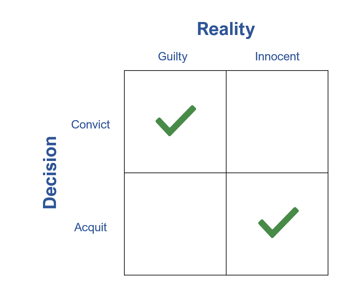
Figure 1: A binary decision (as in jury trials) can be displayed on a 2×2 grid showing the two correct outcomes.
We want to be in the green checkboxes, making the correct decision about someone’s future. Of course, juries can make wrong decisions. Figure 2 illustrates the two errors.
Juries sometimes let the guilty person go free (acquit the guilty; see the lower-left corner of Figure 2). Juries can also convict the innocent. For example, DNA evidence has exonerated some who have been convicted for crimes they didn’t commit. Such stories often make headlines, as we in the U.S. generally see these cases as more significant errors in the justice system. This more egregious error (convicting the innocent) is in the upper-right corner of Figure 2 (four Xs).
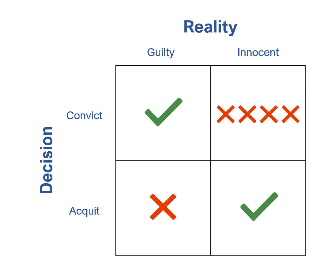
Figure 2: Jury decisions—two ways to be right and two ways to be wrong.
Statistical Decision Making: Type I and Type II Errors
What does this have to do with statistical decision making? It’s not like a jury conducts a chi-square test to reach an outcome. But a researcher, like a jurist, is making a binary decision. Instead of acquitting and convicting, the decision is whether a difference is or is not statistically significant.
As we covered in the earlier article, differences can be computed using metrics such as completion rates, conversion rates, and perceived ease from comparisons of interfaces (e.g., websites, apps, products, and prototypes).
Figure 3 shows how our decisions in hypothesis testing map to juror decisions. Our decision that something is or isn’t significantly different is similar to the jury’s decision to convict or acquit. Likewise, the reality (which we often never know) of whether there’s really a difference is akin to whether the defendant was really innocent or guilty.
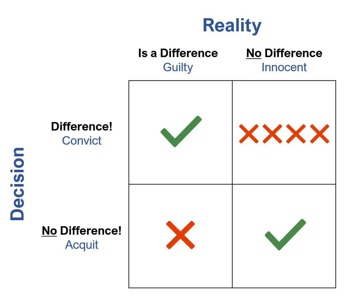
Figure 3: Jury and statistical decisions are similar.
Researchers use the p-value from a test of significance to guide their decisions. If the p-value is low (below alpha), then we conclude the difference is statistically significant and that the result is strong enough to say the difference is real. If this decision is correct, then we’re in the upper-left quadrant of Figure 3 (correct decision). But if there isn’t a difference and we just happened to get an unusual sample, we’re in the upper-right quadrant of Figure 3 (decision error).
On the other hand, if the p-value is higher than alpha, then we would conclude the difference isn’t statistically significant. If the decision matches reality, we’re in the lower-right quadrant of Figure 3 (correct decision). But if there really is a difference that we failed to detect through bad luck or an underpowered experimental design, then we’d be in the lower-left quadrant of Figure 3 (decision error).
Figure 4 shows the creative name statisticians came up with for these two types of errors: Type I and Type II.
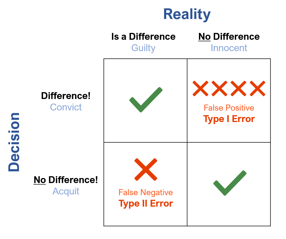
Figure 4: Type I and Type II errors in jury and statistical decisions.
A Type I error can be thought of as a false positive—saying there’s a difference when one doesn’t exist. In statistical hypothesis testing, it’s falsely identifying a difference as real. In a trial, this is convicting the innocent person. Or in thinking of COVID testing, a false positive is a test indicating someone has COVID-19 when they really don’t.
A Type II error is when you say there’s no difference when one exists. It is also called a false negative—failing to detect a real difference. In a trial, this is letting the guilty go free. For COVID testing, that would be someone who has COVID, but the COVID test failed to detect it.
Note that the consequences of Type I and Type II errors can be dramatically different. We already discussed the preference for Type II errors (failing to convict the guilty) over Type I errors (convicting the innocent) in jury trials.
The opposite can be the case for COVID testing, where committing a Type II error is more dangerous (failing to detect the disease, further spreading the infection) than a Type I error (falsely saying someone has the disease, which additional testing will disconfirm). Although even with COVID testing, context matters; false positives may lead to incorrectly quarantining dozens of kids who would lose two weeks of in-school instruction—illustrating the balancing act between Type I and Type II errors.
When researchers use statistical hypothesis testing in scientific publications, they consider Type II errors less damaging than Type I errors. Type I errors introduce false information into the scientific discourse, but Type II errors merely delay the publication of accurate information. In industrial hypothesis testing, researchers must think carefully about the consequences of Type I and Type II errors when planning their studies (e.g., sample size) and choosing appropriate alpha and beta criteria.
Figure 5 includes additional details from the null hypothesis testing framework. We set the Type I error rate (the α criterion) to a tolerable threshold. In scientific publications and many other contexts, the conventional setting is .05 (5%).
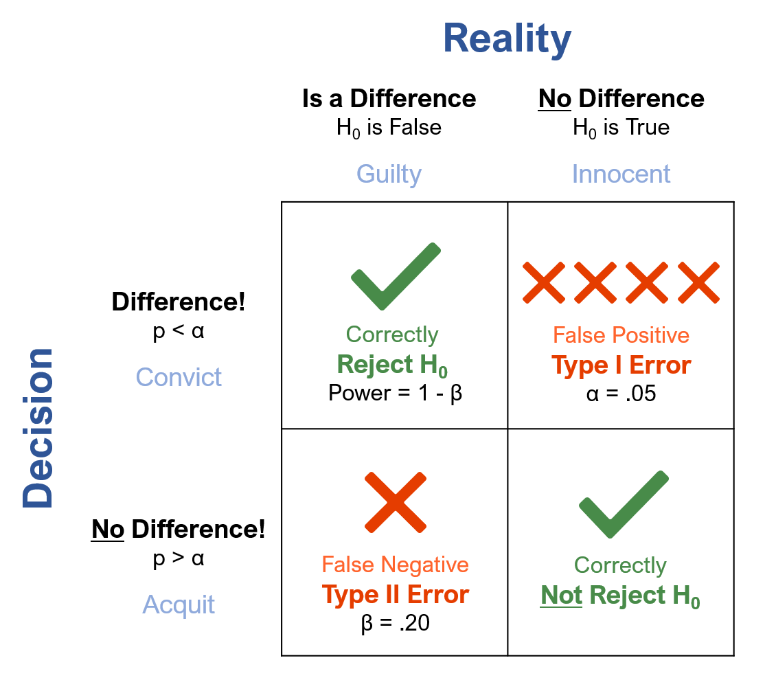
Figure 5: The NHST applied to statistical and jury decisions, with conventional alpha and beta criteria.
We set the Type II error rate at another tolerable threshold, conventionally .20 (20%), four times higher than the Type I error rate. It’s denoted by the Greek letter β in the lower-left corner. This 5% to 20% ratio is the convention used in most scientific research, but as mentioned above, researchers adjust it depending on the relative consequences of the two types of error. (We’ll cover this in more detail in another article.)
You can also see in Figure 5 how the green check marks (the correct decisions) apply to the “truth” of the null hypothesis: there’s one check when there’s really no difference (H0 is true) and we say there’s no difference (lower-right square), and the other when there IS a difference (H0 is false) and we say so (upper-left square).
This framework also guides the development of sample size estimation strategies that balance Type I and Type II errors and holds them to their designated alpha and beta criteria over the long run.
Examples of Decisions
Building on the examples from our previous article on hypothesis testing (all using an alpha criterion of .05), what could go wrong?
1. Rental Cars Ease: 14 users attempted five tasks on two rental car websites. The average SUS scores were 80.4 (sd = 11) for rental website A and 63.5 (sd = 15) for rental website B. The observed difference was 16.9 points (the SUS can range from 0 to 100).
Significance decision. Used a paired t-test to assess the difference of 16.9 points (t(13) = 3.48; p = .004). The value of p was less than .05, so the result was deemed statistically significant.
What could go wrong? A p-value of .004 suggests it isn’t likely that this result occurred by chance, but if there really is no difference, it would be a Type I error (false positive).
2. Flight Booking Friction: 10 users booked a flight on airline site A and 13 on airline site B. The average SEQ score for Airline A was 6.1 (sd = .83) and for Airline B, it was 5.1 (sd = 1.5). The observed difference was 1 point (the SEQ can range from 1 to 7).
Significance decision. The observed SEQ difference was 1 point, assessed with an independent groups t-test (t(20) = 2.1; p = .0499). Because .0499 is less than .05, the result is statistically significant.
What could go wrong? With the p-value so close to the alpha criterion, we’re less confident in the declaration of significance. If there really is no difference, then we’ve made a Type I error (false positive).
3. CRM Ease: 11 users attempted tasks on Product A and 12 users attempted the same tasks on Product B. Product A had a mean SUS score of 51.6 (sd = 4.07) and Product B had a mean SUS score of 49.6 (sd = 4.63). The observed difference was 2 points.
Significance decision. An independent group’s t-test on the difference of 2 points found t(20) = 1.1; p = .28. A p-value of .28 is greater than the alpha criterion of .05, so the decision is that the difference is not statistically significant.
What could go wrong? A p-value of .28 is substantially higher than .05, but this can happen for several reasons, including having a sample size too small to provide enough power to detect small differences. If there is a difference between the perceived usability of Products A and B, then we’ve made a Type II error (false negative).
4. Numbers and Emojis: 240 respondents used two versions of the UMUX-Lite, one using the standard numeric format and the other using face emojis in place of numbers. The mean UMUX-Lite rating using the numeric format was 85.9 (sd = 17.5) and for the face emojis version was 85.4 (sd = 17.1). That’s a difference of .5 points on a 0-100–point scale.
Significance decision. A dependent groups t-test on the difference of .5 points found t(239) = .88; p = .38. Because .38 is larger than .05, the result is not statistically significant.
What could go wrong? Even though the sample size was large and the observed difference was small, there is always a chance that there is a real difference between the formats. If so, a Type II error (false negative) has occurred.
Note that you can’t make both a Type I and a Type II error in the same decision. You can’t convict and acquit in the same trial. If you determine a result to be statistically significant, you might make a Type I error (false positive), but you can’t make a Type II error (false negative). When your result is not significant, the decision might be a Type II error (false negative), but it can’t be a Type I error (false positive).
Summary and Additional Implications
Statistical hypothesis testing can be a valuable tool when properly used. Proper use of hypothesis testing includes understanding the different ways things can go wrong.
The logic of formal statistical hypothesis testing can seem convoluted at first, but it’s ultimately comprehensible (we hope!). Think of it as similar to a jury trial with a binary outcome. There are several key elements:
There are two ways to be right and wrong. When making a binary decision such as significant/nonsignificant, there are two ways to be right and two ways to be wrong.
The first way to be wrong is a Type I error. Concluding a difference is real when there really is no difference is a Type I error (a false positive). This is like convicting an innocent person. Type I errors are associated with statistical confidence and the α criterion (usually .05 or .10).
The second way to be wrong is a Type II error. Concluding a real difference doesn’t exist when one exists is a Type II error (a false negative). This is like acquitting the guilty defendant. Type II errors are associated with statistical power and the β criterion (usually .20).
You can make only one type of error for each decision. Fortunately, you can make only a Type I or a Type II error and not both because you can’t say there’s a difference AND say there’s NO difference at the same time. You can’t convict and acquit for the same decision.
The worse error is context dependent. While the Type I error is the worse error in jury trials and academic publishing (we don’t want to publish fluke results), a Type II error may have a deleterious impact as well (e.g., failing to detect a contagious disease).
Reducing Type I and Type II errors requires an increase in sample size. Reducing the alpha and beta thresholds to unrealistic levels (e.g., both to .001) massively increases sample size requirements. One of the goals of sample size estimation for hypothesis tests is to control the likelihood of these Type I and Type II errors over the long run. We do that by making decisions about acceptable levels of α (associated with Type I errors and the concept of confidence) and β (associated with Type II errors and the concept of power), along with the smallest difference that we want to be able to detect (d).
We rarely know if we’re right. We rarely know for certain if our classification decision matches reality. Hypothesis testing doesn’t eliminate decision errors, but over the long run, it holds them to a specified frequency of occurrence (the α and β criteria).
A nonsignificant result doesn’t mean the real difference is 0. Keep in mind that when an outcome isn’t statistically significant, you can’t claim that the true difference is 0. When that happens, and when the decision you’re trying to make is important enough to justify the expenses, continue collecting data to improve precision until the appropriate decision becomes clear. One way to enhance that clarity is to compute a confidence interval around the difference.
Statistical significance doesn’t mean practical significance. Some statistically significant results may turn out to have limited practical significance, and some results that aren’t statistically significant can lead to practical acceptance of the null hypothesis. We’ll cover this in more detail in our next article on this topic.