Should the sample size n be greater than 30?

If you’ve taken any introductory statistics course or an AP statistics class (or helped your child with it), you’ve encountered the n ≥ 30 rule.

The “magic number 5” rule we’ve written extensively about applies (with its important caveats) to problem discovery for usability testing.

But the n ≥ 30 rule goes beyond usability testing, coming up across disciplines and even in classrooms. It will often be mentioned by skeptical stakeholders and during the peer review process (probably from Reviewer Number 2). Violating it can feel like a methodological sin.

But where does it actually come from? And does it hold up in general and in UX research in particular?

The short answer is that the rule has real statistical roots, but they’re often misunderstood and misapplied.

On One Hand: Arguments for Why Researchers Need n ≥ 30

The n ≥ 30 rule is grounded in two related concerns: whether your statistical analyses will perform accurately with smaller sample sizes (1) when your raw data is normally distributed and (2) when raw data is not normally distributed.

The t-Distribution Converges to Z at about n = 30 for Continuous Data

When learning statistics, you’ll often start with the normal z-distribution for statistical tests. You can use tables or simple formulas to look up z values when making computations. But using the normal z-distribution and tables means you need to know the population standard deviation.

Unfortunately, in applied settings, we rarely know the population standard deviation! Fortunately, the alternative is to use t-distribution tables and computations. They have one additional input compared to z computations, which is the sample size (strictly speaking, n − 1, the degrees of freedom for the t-distributions). However, when the sample size gets to about 30, z and t values converge, so they are roughly the same (see Figure 1).

Consequently, when n is at least 30, you don’t have to deal with somewhat more complicated small-sample statistics. Over time, this statistical footnote calcified into a general-purpose sample size rule.

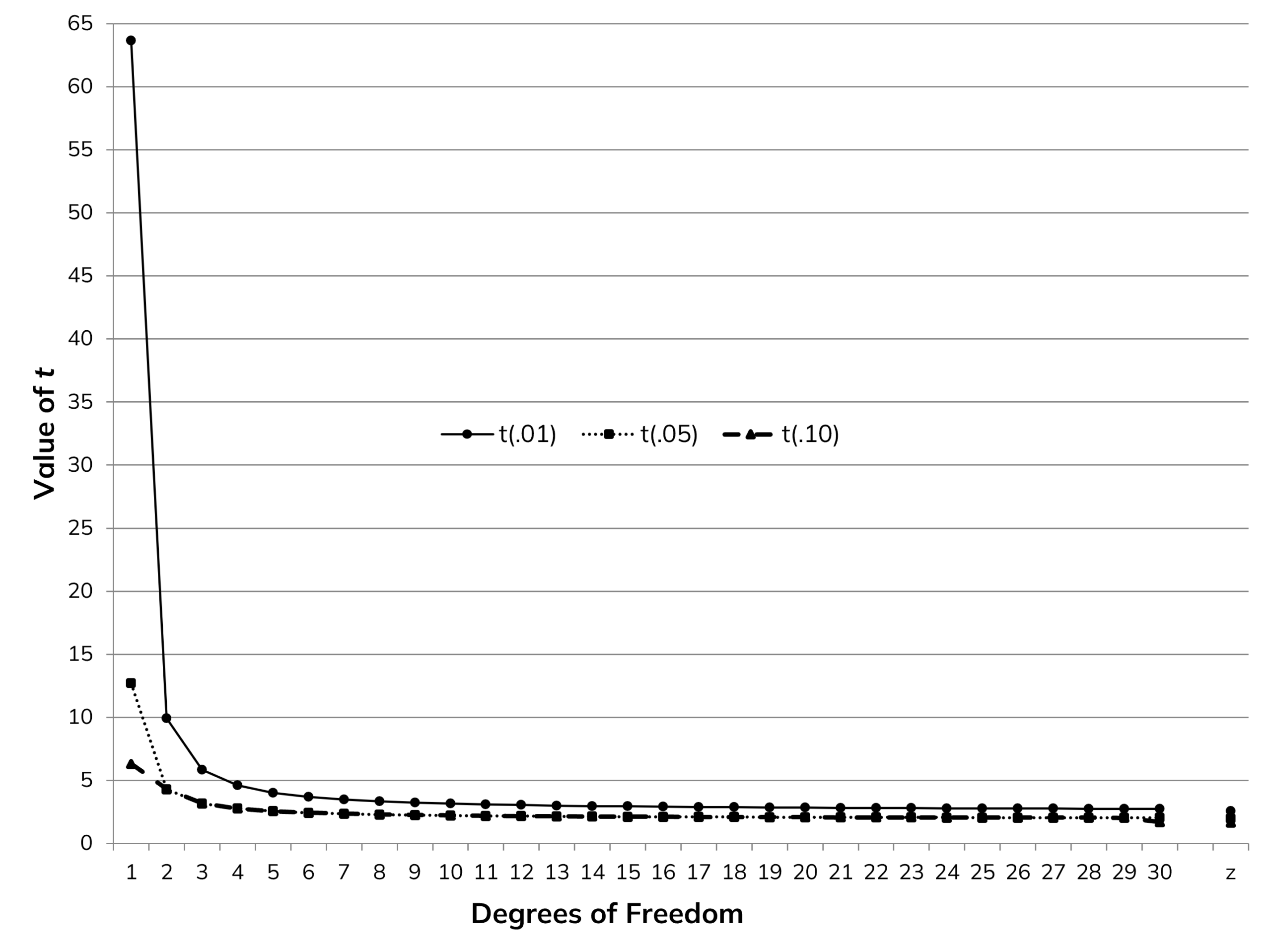
Figure 1: Approach of t to z as a function of degrees of freedom (n − 1).

Traditional “Wald” Confidence Intervals Are Less Accurate at Small Sample Sizes

The n ≥ 30 rule isn’t just for continuous data. It’s also been applied to binary (0/1, yes/no) data. Like the convergence of t to z shown in Figure 1, there is a similar convergence of the binomial distribution to the z-distribution, which becomes approximately normal when n = 30 and the expected proportion is not very close to 0 or 1. The most widely taught method for calculating binomial confidence intervals (the Wald method) grossly understates the width of the true interval when sample sizes are small because it’s based on the z-distribution. We demonstrated the inaccuracy of the Wald method in our 2005 paper using real-world completion rate data. For example, a 95% confidence interval around a completion rate with n = 15 constructed with the Wald method is more like a 72% confidence interval (wildly inaccurate—see below for other findings from that paper).

UX Data Generally Isn’t Normally Distributed

If you’ve ever stared at a histogram of task completion rates, time-on-task, or even SUS scores, you know that raw UX data rarely forms the classic bell curve. Completion rates are binary (0 or 1), usually with more successes than failures. Task times are often-right skewed due to a long tail of slow participants. Likert-scale items such as the Single Ease Question (SEQ^®) tend to cluster toward the top (more scores above the median than below it). As we showed in our article Is UX Data Normally Distributed?, none of these distributions look remotely normal (see Figure 2).

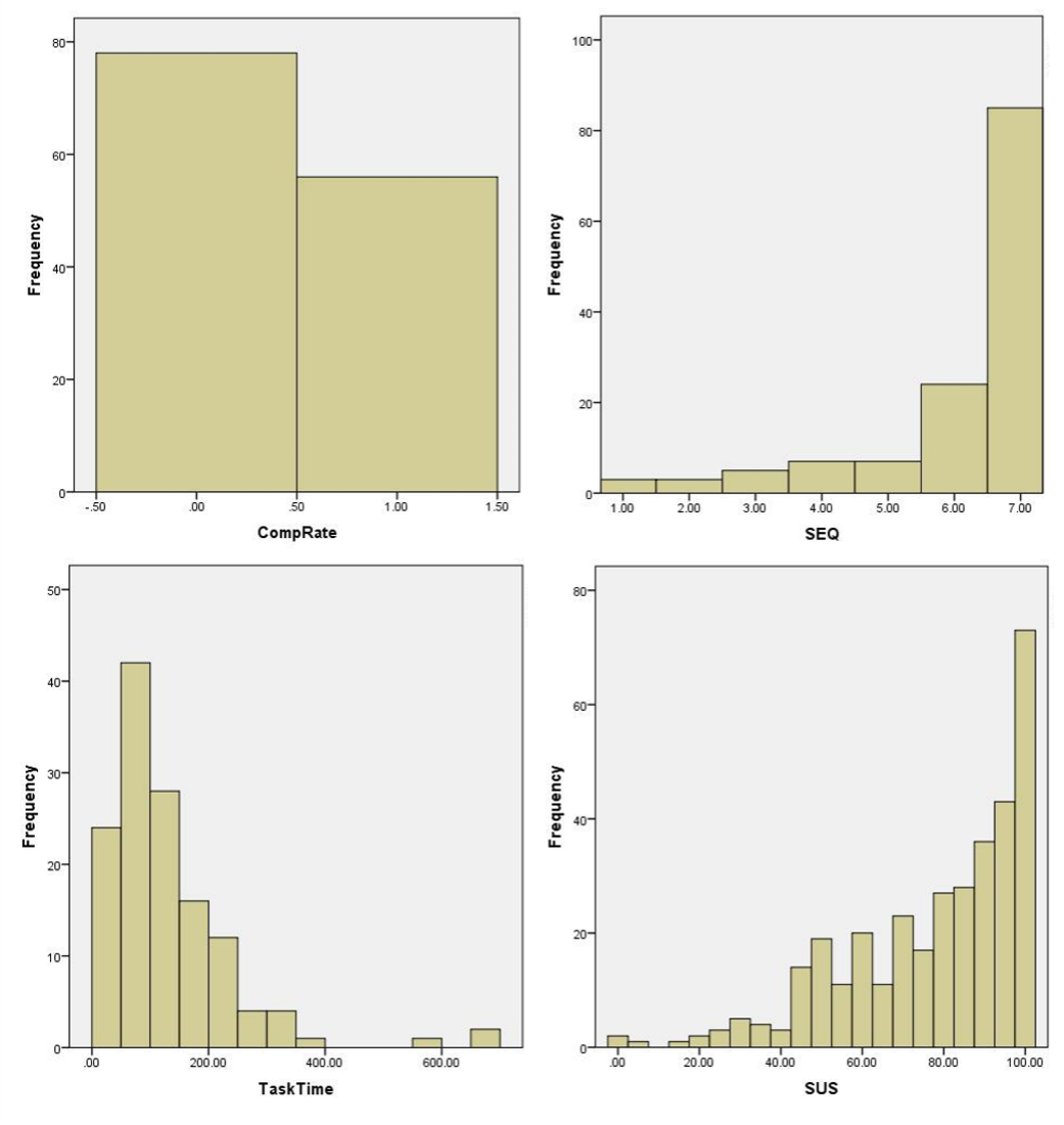
Figure 2: Distributions of four UX metrics showing their non-normal raw distributions.

That might sound alarming. Many statistical tests, such as confidence intervals, t-tests, and ANOVA, assume normality. If the raw data isn’t normal, are those analyses invalid?

On the Other Hand: Arguments Why Sometimes n < 30 Is OK

Fortunately, neither the convergence of t to z nor the non-normality of raw data means confidence intervals or statistical comparison tests are invalid below n = 30. For continuous data, the t-distribution works correctly at any sample size. For binary data, the standard-Wald method can be replaced with better-performing alternatives. And for the normality concern, the Central Limit Theorem (CLT) means the distribution of your raw data matters far less than most researchers assume. This is where the distinction between the distribution of your raw data and the distribution of your sample means becomes critical. We’ll start with the normality issue.

The Central Limit Theorem Solves Most Normality Issues

One of the most important concepts in all of statistics is the CLT. According to the CLT, as the sample size increases, the distribution of the mean becomes more and more normal, regardless of the normality of the underlying distribution.

How quickly does the CLT kick in? Considering a wide variety of distributions, most achieve a normal or near-normal distribution of the means when n is 30, making that a reasonably safe bet when you don’t know anything about the distributions.

For many common UX metrics, however, the distributions of the means approach normality sooner than you’d expect. Using bootstrap simulations on real UX datasets (repeatedly drawing sub-samples and computing means), the sampling distributions of SEQ ratings and SUS scores approach normality by n = 10. Even binomial completion rates (which are maximally non-normal) and completion times approach a normal sampling distribution by n = 20–30 (see Figure 3). But it turns out there’s a fix for even smaller binomial sample sizes (see below).

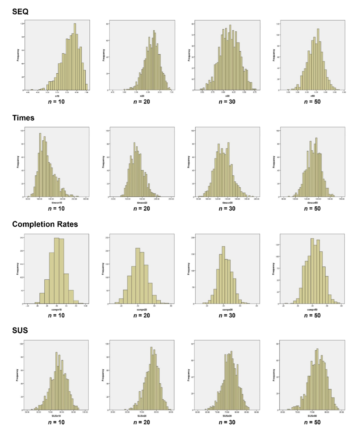
Figure 3: Distributions of the means for four UX metrics with varying sample sizes.

This is why means, t-tests, and confidence intervals work reasonably well even when your raw responses are skewed (e.g., completion times) or bounded (e.g., rating scales).

The t-Distribution Was Built for Small Samples

The deep irony of being advised that “you need 30 to use a t-test” is that the t-distribution was invented specifically for small samples.

In 1899, William S. Gossett (Figure 4), a recent graduate of New College, Oxford with degrees in chemistry and mathematics, became one of the first scientists to join the Guinness brewery.

Figure 4: An anachronistic interpretation of William S. Gossett (Student), adapted from his Wikipedia page photo (public domain) with AI assistance.

As Michael Cowles wrote in his book Statistics in Psychology: An Historical Perspective, “Compared with the giants of his day, he published very little, but his contribution is of critical importance. … The nature of the process of brewing, with its variability in temperature and ingredients, means that it is not possible to take large samples over a long run” (pp. 108–109).

Gossett couldn’t use z-scores because they don’t perform well with small samples. After analyzing the deficiencies of the z-distribution for small-sample statistical tests, he worked out the necessary adjustments as a function of degrees of freedom to produce the t-distribution—published in 1908 under the pseudonym “Student,” because Guinness prohibited employees from publishing. In the work that led to his tables, Gossett performed an early version of Monte Carlo simulations. He prepared 3,000 cards labeled with physical measurements taken on criminals, shuffled them, then dealt them into 750 groups of size 4 (n much smaller than 30).

The point is that the t-distribution was designed precisely to handle small samples correctly. The idea that you need n ≥ 30 even when using the t-distribution contradicts both the history and purpose of the statistic.

Historians of statistics widely regard Gossett’s publication of Student’s t-test as a landmark event. In a letter to Ronald A. Fisher containing an early copy of the t-tables, Gossett wrote, “You are the only man that’s ever likely to use them.”

Gossett got a lot of things right. He certainly got that wrong.

The Wald Method Can Be Fixed with a Simple Adjustment

While binary data generates inaccurate confidence intervals with the standard-Wald method when n < 20–30, there’s a fix. It turns out that a slight adjustment makes even small binomial samples generate accurate confidence intervals. In the same 2005 paper where we demonstrated the problem with the Wald method, we also showed that a simple adjustment brings 95% confidence intervals back to accurate coverage. The adjustment is very close to just adding two successes and two failures to your observed data, then computing a standard-Wald interval around that adjusted proportion. This is now often called the adjusted-Wald method, formalized by work by Agresti and Coull. A small tweak to the math turns an unreliable method into a reliable one, even with small samples.

Our Recommendation: Stats Work Below n = 30 with the Right Approach

When the cost of sampling is high, as it often is, always insisting on at least 30 users regardless of study goals is wasteful at best and infeasible at worst. A more appropriate approach is to use sample size formulas derived from the specific statistical analysis (e.g., confidence interval estimation, significance test), accounting for the data type, expected variability, desired confidence, and target effect size. We’ve published articles on this for several common UX scenarios, for example:

• UX-Lite Sample Sizes for Confidence Intervals
• UX-Lite Sample Sizes for Comparison to a Benchmark
• Sample Sizes for Comparing UX-Lite Scores

Knowing that small samples can work statistically doesn’t tell you how to handle them. The right approach depends on the type of data you’re analyzing:

• Rating scales (SUS, SEQ, SUPR-Q): Use the t-distribution with the correct degrees of freedom for confidence intervals and tests of significance. It was designed for exactly this situation.
• Binary data (completion rates, yes/no): Use adjusted methods (e.g., adjusted-Wald for confidence intervals, N−1 two-proportion method for significance tests), which perform accurately at small samples where standard methods based on the z-distribution break down.
• Time data: For confidence intervals, log-transform the raw data to correct for right-skew, then transform back to the original scale (usually no need to transform for tests of significance, but it is always an option).

When samples are small, the concern shifts from normality and sampling distributions to sensitivity and power—the accuracy of an estimate (confidence intervals) or your ability to detect a true difference when one exists (hypothesis testing).

The procedures work correctly with small samples, but you’re limited to relatively imprecise estimates (confidence intervals) or reliably detecting only large differences (hypothesis tests). Subtle or moderate effects will likely go undetected, not because the statistics are broken but because small samples carry more uncertainty. We cover how to plan for adequate sensitivity and power in all our articles on sample size estimation (e.g., Sample Sizes for Comparing Rating Scale Means). Sometimes a small sample is all you need to achieve your research goal.

This controversy is similar to the “magic number 5” controversy but applied to summative rather than formative research. The “magic number 30” has real empirical rationale, as it’s roughly where the CLT kicks in for a wide variety of distributions and where t converges on z. In practice, however, it’s applied far too rigidly. The appropriate sample size depends on the  distribution, the expected variability, the desired confidence and power, and the minimum effect size you need to detect. A sample of 30 is almost never exactly right for any specific situation.

It isn’t much more complicated to use the t-distribution than the z-distribution, or the adjusted-Wald instead of the Wald method (you just need to account for the sample size). The entire reason the t-distribution was developed was to enable the analysis of small samples. This is just one of the less obvious ways usability practitioners benefit from the science and practice of beer brewing.