 What is the impact if you sample a lot of your population in a survey?
Many statistical calculations—for example, confidence intervals, statistical comparisons (e.g., the two-sample t-test), and their sample size estimates—assume that your sample is a tiny fraction of your population.
But what if you have a relatively modest population size (e.g., IT decision-makers at Fortune 500 companies, fMRI technicians, or Chic-fil-A franchise owners)? These populations don’t comprise millions of people like the U.S. electorate, active Facebook users, or Netflix subscribers.
When the sample size used to compute estimates around a population is large and it meaningfully “depletes” the population, you can use a statistical technique called the finite population correction (FPC), which accounts for the influence of larger sample sizes relative to the population size.
When appropriate, applying the FPC reduces the width of confidence intervals, increases statistical power, and reduces needed sample sizes. It does this by reducing the standard error used in the calculations. The larger the proportion of your sample size in relation to the finite population, the more benefit there is. The benefit becomes noticeable when the sample size is at least 10% of the population.
The Finite Correction Formula
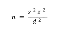
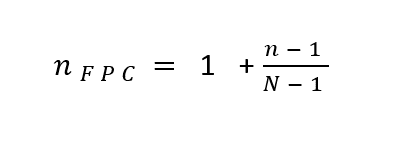
To apply the correction to a finite population, you need the sample size (n) and population size (N):
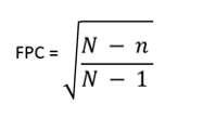
To use the correction, multiply it by the standard error in standard statistical computations (e.g., confidence intervals, tests of significance, sample size estimation). Take a moment to examine this formula. Whenever the sample size is greater than 1, the fraction inside the square root will be less than 1, so its application will always reduce the standard error, making for narrower confidence intervals and smaller sample size requirements.
You might see a variant of the FPC formula with N in the denominator instead of N−1. Statisticians do not necessarily agree about basing the FPC on population variance, in which case the denominator would be N, or on sample variance, in which case the denominator would be N−1 (Cochran, 1977, p. 24). Most modern practitioners use N−1. It doesn’t matter much, because unless N is so small that you’d measure the entire population anyway there would be no practical difference between calculations using N or N−1.
The amount of reduction in confidence intervals and sample sizes depends on how large n is relative to N. When a population is essentially infinite, then N−n and N−1 will be about the same, so the fraction inside the square root will be close to 1. The square root of a number close to 1 is even closer to 1, and there will be essentially no reduction in the standard error. Things get interesting, though, when n is not a trivial proportion of N.
Table 1 shows how large the correction is for different population sizes from 100 to 10,000 based on the sample size.
For example, for populations that are on the large size but still not massive (e.g., 10,000), the correction is relatively insignificant until you get to a sample size of 1,000, which is 10% of the total population. At 10% of the population, you reduce the standard error by about 5%.
For small populations (e.g., 100), you get an impact right away as even a small sample size of 10 represents 10% of the population.
| Sample Size | Pop = 10,000 | Pop = 1,000 | Pop = 500 | Pop = 100 |
|---|---|---|---|---|
| 10 | 99.95% | 99.5% | 99.1% | 95.3% |
| 25 | 99.9% | 98.8% | 97.6% | 87.0% |
| 50 | 99.8% | 97.5% | 95.0% | 71.1% |
| 75 | 99.6% | 96.2% | 92.3% | 50.3% |
| 100 | 99.5% | 94.9% | 89.5% | |
| 250 | 98.7% | 86.6% | 70.8% | |
| 500 | 97.5% | 70.7% | ||
| 1,000 | 94.9% |
Table 1: Effect of FPC on the magnitude of standard errors for various sample sizes and population sizes.
Applying the FPC to Confidence Intervals
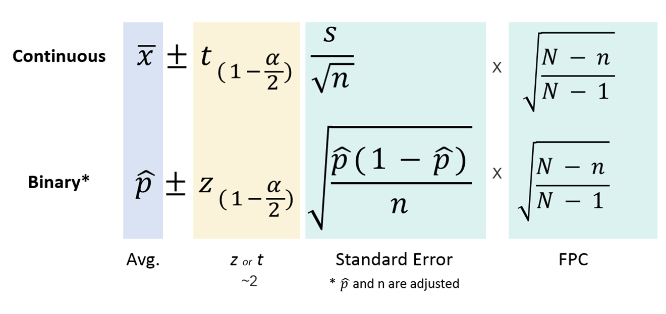
To apply the correction to confidence interval formulas, multiply the correction by the standard error. Figure 1 shows simplified formulas for continuous data (such as rating scales and time) using the t distribution and for binary data (such as completion rates) using the adjusted-Wald formula. It shows the standard error multiplied by the FPC (which is equivalent to multiplying the entire margin of error by the FPC).
Continuous Data
For a sample of 100 SUS scores from a population of 500 (sampling 20% of the population), the FPC is .895 (see Table 1). Table 2 shows unadjusted and FPC-adjusted 95% confidence intervals for a mean System Usability Scale (SUS) of 72.95 with n = 73 and a standard deviation of 23.7.
| 95% CI | Low | High | Width |
|---|---|---|---|
| Unadjusted | 68.2 | 77.7 | 9.4 |
| Adjusted | 68.7 | 77.2 | 8.4 |
Table 2: Example of unadjusted and FPC-adjusted confidence intervals (n = 73, s = 23.7).
The FPC-adjusted result is a confidence interval that’s one point narrower than the unadjusted interval. That translates into more precision (1/9.4 or 10.6% more precision). However, to gain that added precision from the FPC required sampling 20% of the population! That seems like a modest gain for a big sample relative to the population. That’s the nature of the uncertainty still left in the 80% not sampled.
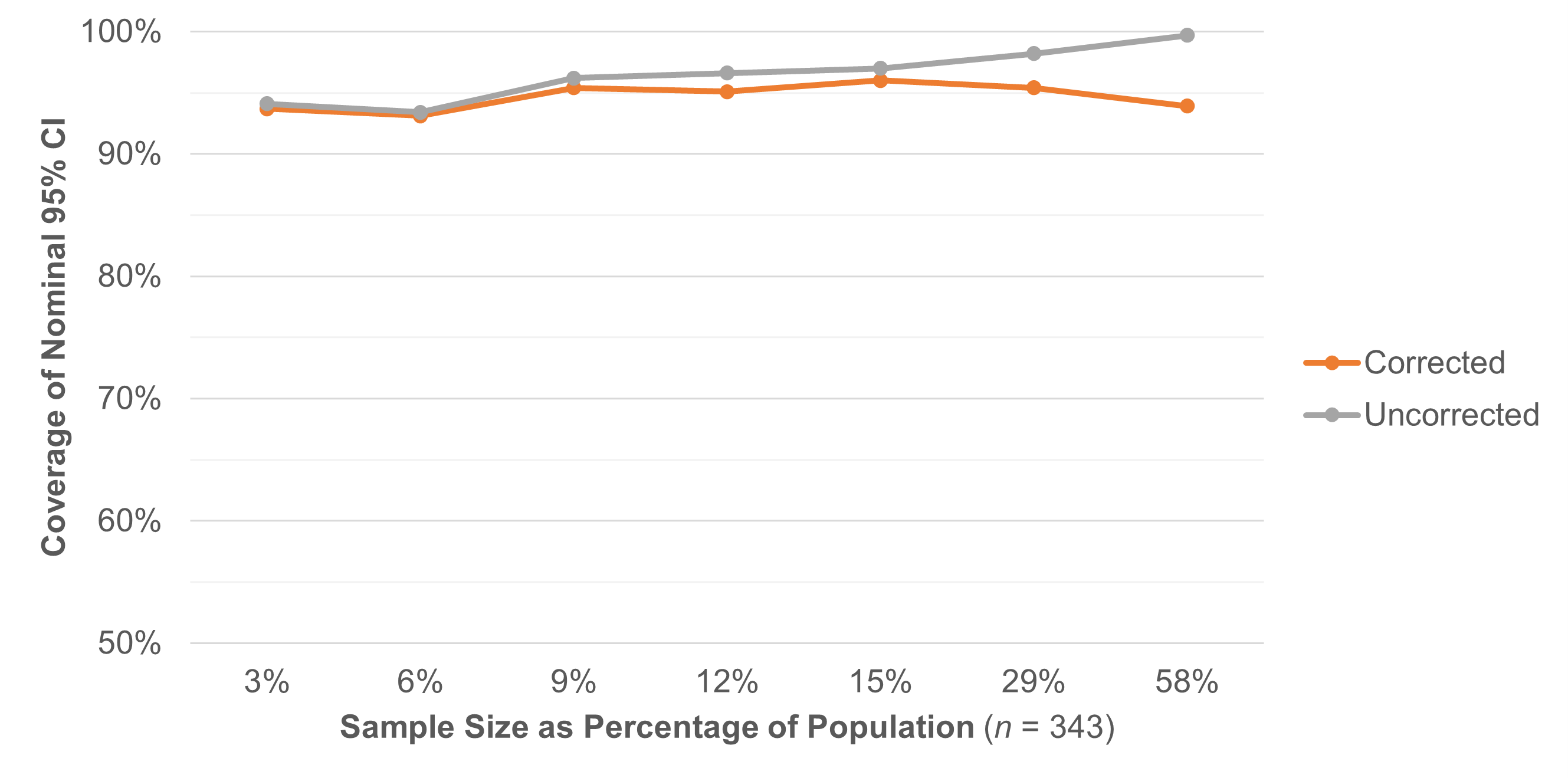
To be sure the correction works for UX data and doesn’t undercorrect or overcorrect, we ran some simulations on large SUS and completion rate datasets. For continuous data, we took SUS scores from a large sample of 343 users and treated this as a population. We then wrote a program to take random sample sizes (without replacement) in increments from 10 to 200 from this population of 343, computing the confidence interval with and without the FPC (Table 3).
| n | % of Pop | FPC | ||
| 10 | 3% | 0.99 | ||
| 20 | 6% | 0.97 | ||
| 30 | 9% | 0.96 | ||
| 40 | 12% | 0.94 | ||
| 50 | 15% | 0.93 | ||
| 100 | 29% | 0.84 | ||
| 200 | 58% | 0.65 | ||
| Avg | ||||
Table 3: Result of taking 1,000 random samples without replacement for each sample size (n from 10 to 200) from a population of 343 SUS scores, tracking the number of times the t-confidence interval (corrected or uncorrected) contained the mean.
Table 3 shows that the FPC-adjusted confidence intervals contained the mean 94.7% of the time compared to 96.5% of the time compared to the uncorrected confidence interval. The difference is most pronounced when there’s a significant depletion (sampling 29% and 58% of the population—see Figure 2). In these cases, as expected, without the correction the confidence intervals are much too wide, containing the mean closer to 99% of the time instead of the specified 95%. This also illustrates how much of the population you need to sample to see the benefits of the FPC.
Binomial Data
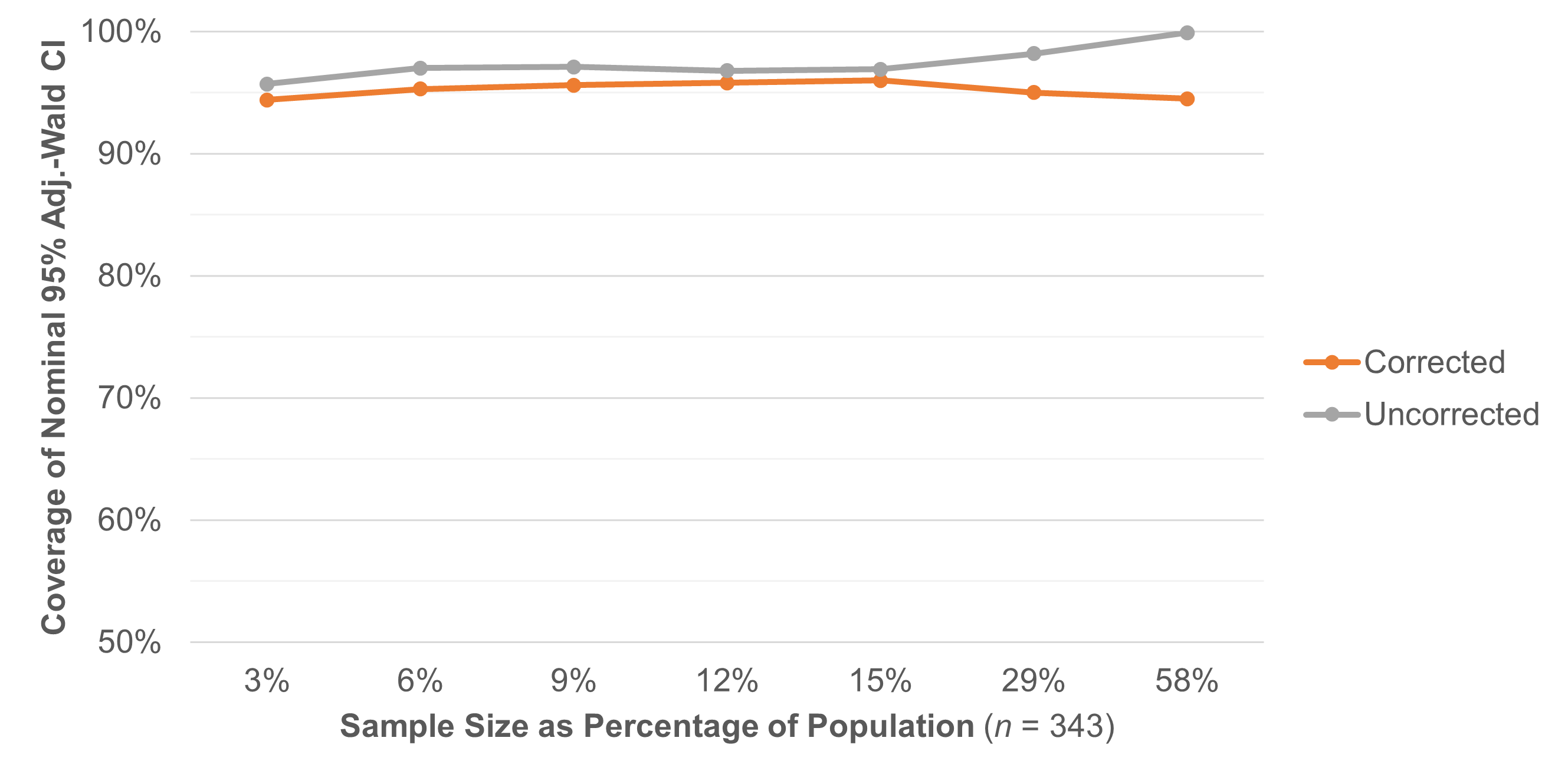
We repeated the resampling exercise, but this time we used binomial data to simulate completion rates. We created populations with a comparable population size to the continuous data example (n = 343) at completion rates of 50%, 75%, 90%, and 95%. We used the same sample sizes from 10 to 200 and computed 95% adjusted-Wald confidence intervals with and without the FPC.
The results in Table 4 and Figure 3 are similar to the SUS results in Table 3 and Figure 2. The corrected binomial confidence interval contained the population completion rate on average 95.2% of the time compared to the uncorrected formula, which had 97.4% coverage (too wide and therefore too conservative by 2.2%). The largest gap in coverage, like the SUS data, is when the sample is a substantial portion of the population (n = 100 and n = 200), where the confidence intervals produced without correction are much too conservative.
| n | ||
| 10 | ||
| 20 | ||
| 30 | ||
| 40 | ||
| 50 | ||
| 100 | ||
| 200 | ||
| Avg | ||
Table 4: Result of taking 1,000 random samples (without replacement) with n from 10 to 200 from a population of 343 completion scores (1s and 0s), tracking the number of times the adjusted-Wald confidence interval (corrected or uncorrected) contained the population proportion.
Applying the FPC to Sample Sizes for Confidence Intervals
For computing sample sizes, we have to solve for the sample size, so the standard error (standard deviation divided by the square root of the sample size) isn’t explicitly represented in the formula. Using the method described in Quantifying the User Experience, the formula for estimating sample sizes is
To apply the correction, divide the computed sample size (n) by
For consistency, we use N−1 in the denominator rather than N. When n = 1, the fraction is 0 so there is no effect on the standard sample size estimate. As n increases, the adjusted sample size estimate decreases.
The impact of the correction formula can be seen in Table 5, which shows the unadjusted sample sizes for generating a 95% confidence interval on binary data with the uncorrected and correct sample sizes at population sizes of 500 and 100.
| Margin of Error (+/−) | (N = 500) | (N = 100) |
|
|---|---|---|---|
| 24% | |||
| 20% | |||
| 17% | |||
| 15% | |||
| 14% | |||
| 13% | |||
| 12% | |||
| 11% | |||
| 10% | |||
| 9% | |||
| 8% | |||
| 7% | |||
| 6% | |||
| 5% | |||
| 4% |
Table 5: Sample size needed for margins of error at a 95% confidence level for uncorrected and corrected sample sizes for the adjusted-Wald confidence interval assuming a proportion of .5 and population sizes of 500 and 100.
For example, the sample size needed to obtain a 5% margin of error on a 95% confidence interval is 381 (uncorrected), but if the population is 500, you need only 276 to reach that level of precision, and if N = 100 you only need 79. This example shows that when a population is small (N = 100) and a substantial amount of the population is being sampled (79%!), there’s still enough uncertainty that the margin of error will be ±5%.
Note that this is the level of uncertainty when binomial variance is maximized (when p = .5). When you expect p to be somewhere in the range of .3 to .7, guidance from aids like Table 5 works well in practice (Cochran, 1977, p. 76–77). If, however, you expect p to have a more extreme value (say, p < .1 or > .9), it is better to estimate the sample size with the formula or use an inverse sampling strategy.
Summary and Discussion
When a sample will significantly deplete your population, you should use the finite population correction (FPC) to improve the accuracy of estimates when computing confidence intervals and in sample size calculations.
FPC really kicks in with 10%+ sample depletion. The FPC tends to have a more meaningful impact on your calculations once the sample size gets above 10% of the population. For anything less, the correction has a minimal effect.
FPC works on continuous and binary data. The effect of FPC is similar for continuous and binary confidence intervals, keeping the coverage of the confidence intervals close to the nominal confidence level regardless of the percentage of the sample size (n) divided by the population size (N). This is especially important when n/N is over 10%.
There is little gain for a lot of depletion. Surprisingly, even with a large depletion of the sample, a fair amount of uncertainty remains when the population variance is high. For example, if N = 100 and n = 79 (79% of the population), the margin of error for a binomial metric such as completion rates will be ±5% (when the completion rate p is expected to be about .50).
Don’t define your population too narrowly. We’ve found some researchers may define their population too narrowly (e.g., only existing nurses who use a product) but then want to generalize their findings to a broader audience (e.g., all future nurses who will use the product). This could lead to errors in the use of FPC if the actual population is much larger than the defined population (i.e., the correction will actually be a miscorrection).
The FPC should apply to significance tests. In this article, we did not specifically examine the effects of FPC on tests of significance (e.g., t-tests), but the math should also be applicable in that context, multiplying standard errors by the square root of (N−n)/(N−1).


")