 Proportional data is common in both UX research and the larger scientific literature.
You can use proportions to help make data-driven decisions just about anywhere: Which design converts more? Which product is preferred? Does the new interface have a higher completion rate? What proportion of users had a problem with registering?
Consequently, you’ll likely want to statistically compare proportions. But what’s the best test to use, especially if the sample size is small?
In 2012, when we published the first edition of Quantifying the User Experience, we provided several decision trees to assist in the selection of appropriate statistical methods for different situations.
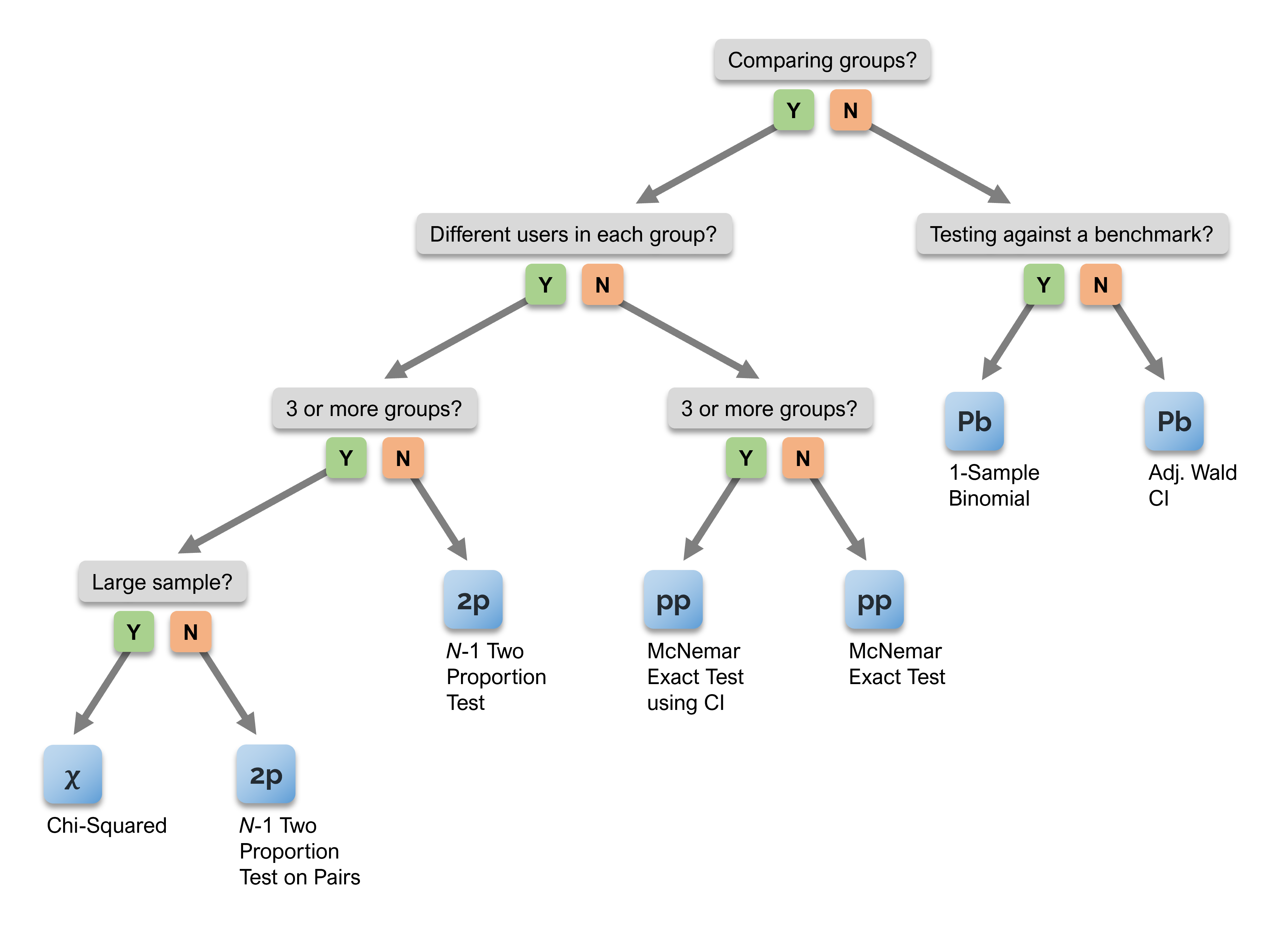
The first decision point is whether the data are binary (a combination of measured 0s and 1s that can be expressed as proportions or percentages) or more continuous (e.g., multipoint rating scales or times).
Figure 1 shows the decision map for binary data. When comparing groups of binary data, the appropriate method depends on whether the experimental design is between-subjects (different users in each group) or within-subjects (same users in each group).
When there are different users in each group and only two groups to compare, the decision tree terminates at the N−1 two-proportion test.
Before we started doing the research for our book, we’d never heard of this statistical test. In this article, we explain what the N−1 two-proportion test is and why we recommend it over the better-known chi-square and Fisher exact (also known as Fisher-Irwin) tests.
Chi-Square Test of Independence
One of the oldest methods (and the one typically taught in introductory statistics books) is the chi-square test, proposed in 1900 by Karl Pearson. It uses an intuitive concept of comparing the observed counts in each group with what you would expect from chance. Because the chi-square test makes no assumptions about the parent population in each group, it’s usually (but not always) classified as a distribution-free nonparametric test. For one of its basic applications, it uses a 2 × 2 table (pronounced two by two) with the nomenclature shown in Table 1 (set up to test the significance of differences in a task’s successful completion rate for two designs).
| Design | Success | Failed | Total |
|---|---|---|---|
| Design A | a | b | m |
| Design B | c | d | n |
| Total | r | s | N |
Table 1: Nomenclature for chi-square test of independence.
The general formula for the chi-square test (which has one degree of freedom) is:
![]()
For example, consider the data in Table 2.
| Design | Success | Failed | Total |
|---|---|---|---|
| Design A | 40 | 20 | 60 |
| Design B | 15 | 20 | 35 |
| Total | 55 | 40 | 95 |
Table 2: Example data for a chi-square test.
If 40 out of 60 (67%) users complete a task on Design A, can we conclude it is statistically different from Design B, where 15 out of 35 (43%) users succeeded? Putting the values in the formula, we get:

The resulting value of chi-square is 5.1406 with one degree of freedom. A convenient way to get the p-value for this result is to use the function =CHIDIST(5.1406, 1), available in Excel and Google Sheets, which gives p = .0234. Using the standard alpha criterion of .05, this indicates that Design A has a significantly higher completion rate.
This works well when sample sizes are fairly large, but not when sample sizes are small enough that the expected number of counts in a cell of the 2 x 2 table is less than 5. This way of conceptualizing the analysis also makes computing a confidence interval around the difference difficult in successful completion rates.
Fisher Exact Test
The Fisher exact test is another way to analyze 2 × 2 tables using a method that Sir Ronald Fisher published in 1935. Rather than using a simple formula and associated statistical distribution to compute a value for p, the Fisher exact test is an early example of a type of randomization test known as a permutation test. For this reason, Fisher exact tests are analyzed using software that is available in the major statistical packages, online calculators, or programmed in Excel.
Even though it does not have the sample size limitation of the chi-square test, like other exact randomization tests, its p-values tend to be slightly conservative (higher than they should be). If we analyze our sample data with our online Fisher exact test, the resulting p-value is .0315, still significant but slightly larger than the .0234 from the chi-square test. It also shares the limitation of the chi-square test because it doesn’t easily allow for the calculation of confidence intervals around observed differences.
Two-Proportion Test
A more direct way to compare two proportions is with the two-proportion test. The formula for the two-proportion test is
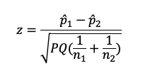
where
- The numerator is the difference between the two sample proportions (x1/n1 − x2/n2)
- P is the combined proportion: (x1 + x2)/(n1 + n2)
- Q is 1 − P
Despite its very different form, this test is mathematically equivalent to the chi-square test.
For example, if we set up our example data in this form, we get
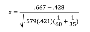
After doing the arithmetic, z = .2381/.1050 = 2.267. To get the p-value for z, you can use the following formula in Excel or Google Sheets: =2*(1-NORMSDIST(2.267)), which is .0234—the same value we got with the chi-square test. Also note that this value of z is the square root of the corresponding chi-square value, another indication of their mathematical equivalence. Isn’t math fun?
Despite its conceptual advantages over the 2 × 2 chi-square test, the two-proportion test has the same sample size limitation, so it should only be used when there are at least ten successes and ten failures in each sample.
N-1 Two-Proportion Test
So, in 2012, this is where we were until Jeff found an article (published in the journal Statistics in Medicine) that focused on the best way to analyze these types of data when sample sizes are small (“Chi-squared and Fisher-Irwin tests of two-by-two tables with small sample recommendations,” Ian Campbell, 2007).
Campbell reviewed the history of analysis of 2 × 2 tables, including a little-known variant of the chi-squared test in which N is replaced by N−1 (published by Egon Pearson, son of Karl Pearson, in 1947). Campbell used computer-intensive techniques to compare seven approaches to the analysis of 2 × 2 tables (including the Yates correction for continuity) and found that they corresponded closely when sample sizes were very large, but not when they were small. He concluded that the optimum method was the N−1 chi-squared test with regard to the precision of the p-values and power of the test, as long as the minimum expected number in a cell was at least 1 (which is almost always the case). For those rare cases when this requirement isn’t met, he recommended using the Fisher exact test.
Large-Sample Example
Applying this N−1 modification to the two-proportion test and continuing our fairly large-sample example get us this:

As N becomes larger, the ratio of N−1 over N gets closer and closer to 1, so the effect of this modification on resulting p-values will be larger when the sample size is smaller.
For the sample data we’ve been analyzing, if we multiply 2.267 by the square root of 94/95, we get z = 2.255, which has a slightly increased p-value of .0241. Recalculating the chi-square example with N−1 gets a value of 5.087, which also has p = .0241 (and the square root of 5.087 is 2.255).
Small-Sample Example
Consider an example with a smaller sample size, shown in Table 3:
| Design | Success | Failed | Total |
|---|---|---|---|
| Design A | 11 | 1 | 12 |
| Design B | 5 | 5 | 10 |
| Total | 16 | 6 | 22 |
Table 3: Small-sample example.
The resulting p-values for the standard chi-square test (equivalent to the two-proportion test), the Fisher exact test, and the N−1 two-proportion test (equivalent to the N−1 chi-square test) are
- Chi-Square Test: .029
- Fisher Exact Test: .056
- N−1 Two-Proportion Test: .033
Confidence Interval
For confidence intervals around the difference of two proportions, we use the method published by Agresti and Caffo (2000 [PDF]). The first step is to adjust the observed proportions by adding z2/4 to the numerator and z2/2 to the denominator, where the value of z is determined by the desired level of confidence (e.g., for 95% confidence, z = 1.96; for 90% confidence, z = 1.645). This is the formula for the margin of error (MoE):
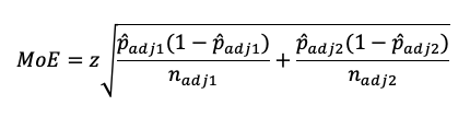
The confidence interval is the difference between the adjusted proportions plus/minus the MoE.
For the small-sample example, the observed difference between proportions is 41.7%, the difference between adjusted proportions is 35.9%, and the lower and upper limits of the 95% confidence interval are 2.2% to 69.7% (a large confidence interval, but n is relatively small).
For the larger-sample example, the observed difference between proportions is 23.8%, the difference between adjusted proportions is 22.9%, and the lower and upper limits of the 95% confidence interval are 3.1% and 42.8% (still a wide interval, but narrower than the small-sample example).
Summary and Discussion
Before 2007, the standard practice when analyzing 2 × 2 tables to assess the statistical significance of the difference in proportions was to use the standard chi-square test with larger sample sizes and the Fisher exact test with smaller sample sizes.
In 2007, Campbell published assessments of the accuracy and power of different methods for analyzing 2 × 2 tables. He found that in most cases, even with small sample sizes, the best performing method was a little-known variation of the chi-square test in which the total sample size N was replaced by N−1.
A mathematically equivalent method that produces a z score instead of a chi-square value with one degree of freedom is the N−1 two-proportion test. Except in the rare case when the expected number in a cell of the 2 × 2 table will be less than 1, we recommend analyzing differences in proportions with the N−1 two-proportion test for several reasons:
- In UX research, it’s often easier to think in terms of completion rates or conversion rates (measured as proportions and expressed as percentages) rather than the number of users who succeed or fail.
- It works well across a wide range of sample sizes.
- This method uses the more familiar and readily available normal (z) distribution as the reference for determining p-values (and without the need to worry about degrees of freedom).
- The confidence interval formula uses the difference between the two proportions and makes for an easier transition in computation and understanding.