 Are customers more satisfied this quarter than last quarter?
Do users trust the brand less this year than last year?
Did the product changes result in more customers renewing their subscriptions?
When UX researchers want to measure attitudes and intentions, they often ask respondents to complete multipoint rating scale items, which are then compared with changes in other samples (e.g., over time) in surveys or benchmark studies.
To compute sample sizes for comparing means, we need some inputs and assumptions.
A common question is what sample size is needed to compare rating scale means from two samples.
All sample size calculations require an estimate of the variability of the metric, expressed as a standard deviation. This is easy for binary and NPS data because their standard deviations can be generated from their proportions. For continuous data, you need some idea of the standard deviation, for example, by analyzing normal and uniform distributions, using a fraction of the maximum range of a scale, or basing an estimate on historical data. Of these various methods, historical data is the most accurate.
In an earlier article, we showed how to calculate sample sizes when computing confidence intervals (no comparisons) around mean ratings or when comparing a mean rating to a benchmark. In this article, we’ll use the same standard deviations from our large dataset of 100,000 individual rating scale responses and numerous standardized UX questionnaires to compute the sample size when comparing individual rating scales (e.g., five- or seven-point items) or multi-item questionnaires: comparison of two means collected from the same people (within-subjects) and comparison of two means collected from different groups of people (between-subjects).
What Drives Sample Size Requirements for Comparing Rating Scale Means?
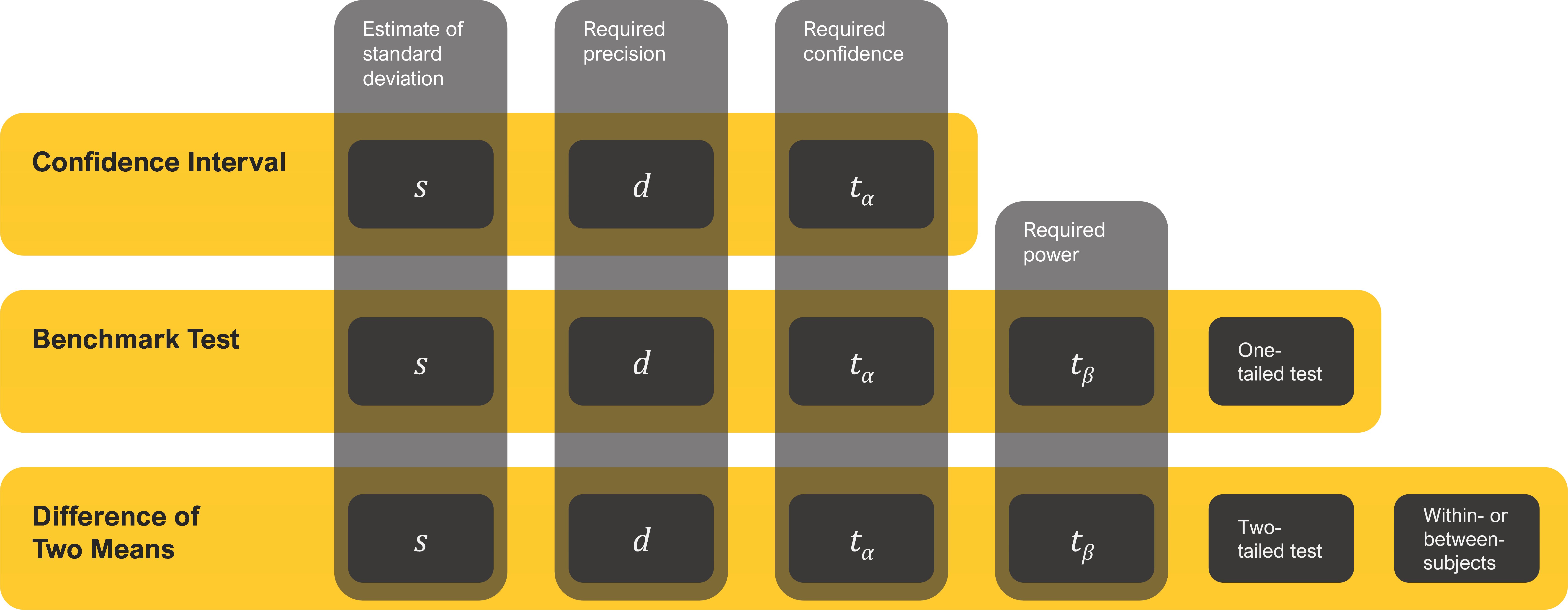
You need to know six things to compute the sample size when comparing means. The first three are the same elements required to compute the sample size for a confidence interval.
- An estimate of the rating scale standard deviation: s
- The required level of precision (using points or percentages): d
- The level of confidence (typically 90% or 95%): tα
Sample size estimation for comparing a mean against a set benchmark or two means against one another requires two additional considerations:
- The power of the test (typically 80%): tβ
- The distribution of the rejection region (one-tailed for benchmark tests, two-tailed for means)
Comparing two means requires one more consideration:
- Whether it’s a within- (same people in each sample) or between-subjects (different people in each sample) study
Figure 1 illustrates how the number of sample size drivers increases and changes from confidence intervals (the simplest with three drivers) to benchmark testing (five drivers) to tests of two means (six drivers).
Quick Recap of Power and Tails (Rejection Regions)
The power of a test refers to its capability to detect a specified minimum difference between means (i.e., to control the likelihood of a Type II error). The number of tails refers to the distribution of the rejection region for the statistical test. In the vast majority of cases, comparisons of two SUS means should use a two-tailed test. For more details on these topics, see the previous article on SUS benchmark testing.
Quick Recap of Typical, Low, and High Standard Deviations for Multipoint Rating Scales and Multi-Item Questionnaires
From our analyses of historical standard deviations and other approaches to estimating unknown standard deviations, we found a good estimate of the typical (50th percentile) standard deviation of an individual rating scale is about 25% of the maximum range of the scale (e.g., 1 point on a five-point scale) and a more conservative (75th percentile) estimate is about 28% of the maximum range of the scale (e.g., 1.12 points on a five-point scale). A good (50th percentile) estimate of the typical standard deviation of a multi-item questionnaire is about 20% of the maximum range of the scale (e.g., 20 points on a 0–100-point scale) which, coincidentally, is a reasonable estimate of a liberal (25th percentile) standard deviation for individual rating scales (e.g., .8 point on a five-point scale).
Sample Size Formulas and Tables for Comparing Means
In a within-subjects study, you compare the means of scores that are paired because they came from the same person (assuming proper counterbalancing of the order of presentation of experimental conditions). In a between-subjects study, you compare the means of scores that came from different (independent) groups of participants. Each experimental design has its strengths and weaknesses. The sample size estimation process is different for each.
Note that the simple sample size formulas in this article work reasonably well when the sample size n is greater than 20, but underestimate the requirements when n is smaller than 20. To get the most precise estimate we can, the entries in this article’s tables have been computed using the iterative method described in Quantifying the User Experience.
Also, we expect these sample size estimates for rating scales to be very accurate when item means are close to the midpoint and reasonably accurate until means get close to an endpoint. Because the standard deviations for rating scales approach 0 as means approach a scale endpoint, the actual sample size requirements for extreme means will be smaller than those in the tables. This isn’t a problem when the cost of additional samples is small, but when that cost is high, consider running a pilot study to get an estimate of the actual standard deviation rather than using the tables.
Standardizing Ratings to a 0–100-Point Scale
To standardize the tables in this article so they work for any number of points in a multipoint scale or multi-item questionnaire, we interpolated the values in the Effect Size columns in the following sample size tables to a 0–100-point scale. Table 1 shows how these effect sizes (unstandardized mean differences) correspond to equivalent mean differences on five-, seven-, and eleven-point scales. For example, a mean difference of 20 points on a 0–100-point scale is equivalent to a difference of 0.8 on a five-point scale (endpoints from 1 to 5), 1.2 on a seven-point scale (endpoints from 1 to 7), or 2.0 on an eleven-point scale (endpoints from 0 to 10).
| 0–100-pt Scale | Five-pt Scale | Seven-pt Scale | Eleven-pt Scale |
|---|---|---|---|
| 50 | 2.00 | 3.00 | 5.00 |
| 40 | 1.60 | 2.40 | 4.00 |
| 30 | 1.20 | 1.80 | 3.00 |
| 20 | 0.80 | 1.20 | 2.00 |
| 15 | 0.60 | 0.90 | 1.50 |
| 12 | 0.48 | 0.72 | 1.20 |
| 10 | 0.40 | 0.60 | 1.00 |
| 9 | 0.36 | 0.54 | 0.90 |
| 8 | 0.32 | 0.48 | 0.80 |
| 7 | 0.28 | 0.42 | 0.70 |
| 6 | 0.24 | 0.36 | 0.60 |
| 5 | 0.20 | 0.30 | 0.50 |
| 4 | 0.16 | 0.24 | 0.40 |
| 3 | 0.12 | 0.18 | 0.30 |
| 2 | 0.08 | 0.12 | 0.20 |
| 1 | 0.04 | 0.06 | 0.10 |
Comparing Two Within-Subjects Means
The basic sample size formula for a within-subjects study is the same as the one used for confidence intervals and tests against a benchmark:
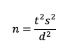
where s is the standard deviation, t is the summed t-value for the desired level of confidence (tα) AND power (tβ), and d is the target for the effect size (the smallest difference in means that you need to be able to detect).
For details on setting the values for tα and tβ in this experimental design, see “Sample Sizes for Comparing SUS Scores.” In contrast to benchmark tests, a comparison of means is two-tailed because you want to detect the difference regardless of which mean is larger, so the appropriate value of tα in the formula should be two-sided (e.g., when n > 20, set tα to 1.98 for 95% confidence or 1.645 for 90% confidence). For 80% power (and n > 20), the value of tβ remains 0.842.
Table 2 shows the sample size estimates for within-subjects t-tests for various effect sizes (minimally detectable differences between the means, percentage points for a McNemar test of discordant proportions, scale points for rating scales), three magnitudes of rating scale standard deviations (s = 20, suitable for multi-item questionnaires; s = 25, suitable for individual multipoint rating items; s = 28, suitable for individual multipoint rating items that are suspected to be more variable than the typical item), variable standard deviation for the within-subjects binary metric (s = 56–75% from the effect sizes of 50% to 1%), 95% confidence (i.e., setting the Type I error to .05), and 80% confidence (i.e., setting the Type II error to .20). The only difference in Table 3 is that confidence is 90% (i.e., Type I error set to .10), a common criterion for industrial research.
Unlike most binomial sample size estimation processes, sample sizes for the McNemar test are affected by the sum of the discordant proportions that the test compares. (For more information, see our article on sample sizes for testing differences between two dependent proportions.) The binary sample sizes in Tables 2 and 3 use our conservative reasonable estimate for discordant proportions (75th percentile value of .28) for the binary metric sample sizes.
Unlike the McNemar test, which is relatively insensitive and therefore needs fairly large sample sizes to reliably detect even large effect sizes, the t-test for comparison of within-subjects means is very sensitive, so the sample sizes for rating scales are 11–19% of those for within-subjects binary metrics.
| Effect Size | Binary Metric s = 56–75% | 0–100-Point Rating Scale, s = 20 | 0–100-Point Rating Scale, s = 25 | 0–100-Point Rating Scale, s = 28 |
|---|---|---|---|---|
| 50(%) | 22 | 2 | 3 | 4 |
| 40(%) | 27 | 3 | 5 | 6 |
| 30(%) | 47 | 5 | 8 | 9 |
| 20(%) | 107 | 10 | 15 | 18 |
| 15(%) | 192 | 16 | 24 | 30 |
| 12(%) | 302 | 24 | 36 | 45 |
| 10(%) | 436 | 34 | 51 | 64 |
| 9(%) | 539 | 41 | 63 | 78 |
| 8(%) | 683 | 51 | 79 | 99 |
| 7(%) | 893 | 67 | 103 | 128 |
| 6(%) | 1217 | 90 | 139 | 173 |
| 5(%) | 1754 | 128 | 199 | 249 |
| 4(%) | 2743 | 199 | 309 | 387 |
| 3(%) | 4880 | 351 | 548 | 686 |
| 2(%) | 10985 | 787 | 1229 | 1541 |
| 1(%) | 43950 | 3142 | 4908 | 6156 |
For example, to detect a difference of 10 points between two within-subjects means with 95% confidence, start in the column in Table 2 labeled Effect Size and move down to the row starting 10(%). The column labeled “Binary Metric, s = 56–75%” is the sample size needed for a binary metric with that margin of error which, assuming a relatively large but reasonable variance, would be 436. Using the typical standard deviation estimate for rating scales (25% of range) would reduce the sample size to 51. The sample size for rating scales saves the expense of 385 participants and is about 12% of the sample size for binary metrics!
| Effect Size | Binary Metric s = 56–75% | 0–100-Point Rating Scale, s = 20 | 0–100-Point Rating Scale, s = 25 | 0–100-Point Rating Scale, s = 28 |
|---|---|---|---|---|
| 50(%) | 17 | 2 | 2 | 3 |
| 40(%) | 21 | 2 | 4 | 5 |
| 30(%) | 37 | 5 | 6 | 7 |
| 20(%) | 84 | 8 | 12 | 14 |
| 15(%) | 151 | 13 | 19 | 24 |
| 12(%) | 238 | 19 | 29 | 36 |
| 10(%) | 343 | 27 | 41 | 50 |
| 9(%) | 425 | 33 | 50 | 62 |
| 8(%) | 538 | 41 | 62 | 78 |
| 7(%) | 704 | 52 | 81 | 101 |
| 6(%) | 959 | 71 | 109 | 137 |
| 5(%) | 1382 | 101 | 157 | 196 |
| 4(%) | 2161 | 157 | 244 | 305 |
| 3(%) | 3844 | 277 | 431 | 541 |
| 2(%) | 8653 | 620 | 968 | 1214 |
| 1(%) | 34619 | 2475 | 3866 | 4849 |
Comparing Two Between-Subjects Means
The sample size formula for a between-subjects study is the basic equation multiplied by 2:
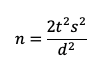
where s is the standard deviation, t is the summed t-value for the desired level of confidence (tα) AND power (tβ), and d is the target for the effect size (the critical difference). For details on setting the values for tα and tβ in this experimental design, see “Sample Sizes for Comparing SUS Scores.”
| Effect Size | Binary Metric, s = 50% | 0–100-Point Rating Scale, s = 20 | 0–100-Point Rating Scale, s = 25 | 0–100-Point Rating Scale, s = 28 |
|---|---|---|---|---|
| 50(%) | 13 | 4 | 6 | 7 |
| 40(%) | 22 | 6 | 8 | 9 |
| 30(%) | 41 | 9 | 13 | 15 |
| 20(%) | 95 | 17 | 26 | 32 |
| 15(%) | 171 | 30 | 45 | 56 |
| 12(%) | 270 | 45 | 70 | 87 |
| 10(%) | 390 | 64 | 100 | 125 |
| 9(%) | 482 | 79 | 123 | 154 |
| 8(%) | 610 | 100 | 155 | 194 |
| 7(%) | 798 | 130 | 202 | 253 |
| 6(%) | 1087 | 176 | 274 | 343 |
| 5(%) | 1567 | 253 | 394 | 494 |
| 4(%) | 2450 | 394 | 615 | 771 |
| 3(%) | 4358 | 699 | 1092 | 1369 |
| 2(%) | 9808 | 1571 | 2454 | 3078 |
| 1(%) | 39241 | 6281 | 9813 | 12309 |
| Effect Size | Binary Metric, s = 50% | 0–100-Point Rating Scale, s = 20 | 0–100-Point Rating Scale, s = 25 | 0–100-Point Rating Scale, s = 28 |
|---|---|---|---|---|
| 50(%) | 10 | 4 | 5 | 5 |
| 40(%) | 17 | 5 | 6 | 8 |
| 30(%) | 32 | 7 | 10 | 12 |
| 20(%) | 75 | 14 | 21 | 26 |
| 15(%) | 135 | 23 | 36 | 45 |
| 12(%) | 213 | 36 | 55 | 69 |
| 10(%) | 307 | 51 | 79 | 98 |
| 9(%) | 380 | 62 | 97 | 121 |
| 8(%) | 481 | 79 | 122 | 153 |
| 7(%) | 629 | 102 | 159 | 199 |
| 6(%) | 857 | 139 | 216 | 271 |
| 5(%) | 1234 | 199 | 311 | 389 |
| 4(%) | 1930 | 311 | 484 | 607 |
| 3(%) | 3433 | 551 | 860 | 1079 |
| 2(%) | 7726 | 1238 | 1933 | 2425 |
| 1(%) | 30911 | 4947 | 7730 | 9696 |
All other things being equal, between-subjects comparisons require a much larger sample size than within-subjects comparisons due to the combination of dealing with two standard deviations (assumed to be equal to keep the formula simple) and because the formula produces the sample size for one group, needing to double that number when comparing two groups (and tripling it if there will be three independent groups, and so on).
Returning to the previous example (detection of a difference of 10 points with 95% confidence), in Table 2, the sample size needed to detect a within-subjects difference of 5 points for a rating scale with the typical standard deviation (s = 25) is 51. For a comparable between-subjects comparison (Table 5), the sample size for one group is 79, so the total sample size for two groups is 158—roughly three times the within-subjects sample size (but only about a quarter the sample size needed for a binary metric). Given this, you might wonder why anyone would use a between-subjects design, but the within/between decision is more complicated than just comparing sample sizes.
A Few More Examples
Single eleven-point item. Suppose you’ve created a new eleven-point (0–10) item to measure the likelihood that a customer will defect (stop using your product and start using a competitor’s), such that the higher the rating, the more likely the customer will defect. You want to test whether there is a difference in the ratings of customers who have been with you for more than a year versus those who have been with you for less than six months (two independent groups). You want a sample size large enough to detect a difference as small as 1 on the eleven-point scale. You decide to reduce the risk of having more variability than expected, so you use the 75th percentile standard deviation from our historical data (28% of the range of the scale) and test with 95% confidence and 80% power.
Start with Table 1 to see what effect size to use in Table 4 (95% confidence, between-subjects). A difference of 1 on an eleven-point scale corresponds to a difference of 10 on a 0–100-point scale. The entry in Table 4 for s = 28 and an effect size of 10 indicates the sample size (n) for each group should be 125 (total of 250 for two groups). In summary:
- Type of scale: eleven-point item
- Experimental design: Between-subjects
- Confidence: 95%
- Power: 80%
- Standard deviation: 28% of scale range
- Effect size: 1 point on an eleven-point scale (10 points on a 0–100-point scale)
- Sample size: 125 per group for a two-group total of 250
Single five-point item. For a new five-point (1–5) item that measures the clarity of filter designs on a commercial website, assume you want to know the sample size requirement for comparing participants’ ratings of two websites that were presented in counterbalanced order to each participant (within-subjects) assuming a typical standard deviation (25% of the range of the scale) with 90% confidence, 80% power, and an effect size of 1/5 of a point (.20) on the five-point scale.
Start with Table 1 to see what effect size to use in Table 3 (90% confidence, within-subjects). For a five-point scale, a difference of .20 corresponds to 5 points on a 0–100-point scale. The sample size in Table 3 for s = 25 and an effect size of 5 is n = 157. In summary:
- Type of scale: five-point item
- Experimental design: Within-subjects
- Confidence: 90%
- Power: 80%
- Standard deviation: 25% of scale range
- Effect size: .20 points on a five-point scale (5 points on a 0–100-point scale)
- Sample size: 157
Multi-item questionnaire. What if you have three new seven-point items that measure different aspects of website attractiveness, and you plan to report scores for this questionnaire based on averaging the three ratings and then interpolating the values to a 0–100-point scale for easier interpretation? You want to know the sample size requirement for 90% confidence and 80% power using the typical standard deviation for multi-item questionnaires (20% of the scale range) that will indicate statistical significance when the difference in means is at least 7 points. Each participant will see only one website (between-subjects).
Because the scale in this example ranges from 0 to 100, you can start directly in Table 5 (90% confidence, between-subjects). The sample size for an effect size of 7 when s = 20 is n = 102 for one group, so the sample size for two groups is 204. In summary:
- Type of scale: Multi-item questionnaire
- Experimental design: Between-subjects
- Confidence: 90%
- Power: 80%
- Standard deviation: 20% of scale range
- Effect size: 7 points on a 0–100-point scale
- Sample size: 102 per group for a two-group total of 204
Summary and Takeaways
What sample size do you need when comparing rating scale means? To answer that question, you need several types of information, some common to all sample size estimation (confidence level to establish control of Type I errors, standard deviation, and margin of error or critical difference), others unique to statistical hypothesis testing (one- vs. two-tailed testing, setting a level of power to control Type II errors), and for comparison of means, whether the experimental design will be within- or between-subjects.
The “right” sample size depends on the research details. If accurate estimates of binary metrics are a critical part of your research, use the sample sizes in the binary metrics column in the tables because those sample sizes will be more than adequate for your rating scale analyses. If your primary analyses will be rating scales, in most cases, you can use the “s = 25” column. If you have concerns that your standard deviations might be larger than average, use the “s = 28” column. If your primary analyses will be multi-item questionnaires, it’s reasonable to use the “s = 20” column.
Using rating scale standard deviations over binary calculations significantly reduces sample sizes. If your primary measure in a survey or benchmark study is a rating scale, using sample size calculations for rating scales instead of using binary data at maximum variance provides significant savings. The difference between sample size requirements for binary metrics and rating scales depends on whether the experimental design is within- or between-subjects. For between-subjects, sample sizes for binary metrics are two to four times larger than those for rating scales with typical variability (25% of the scale range). When the design is within-subjects, the difference is greater—from five to nine times larger.
Balance statistics and logistics. When planning a study, these tables help researchers balance statistics and logistics. The math for a high level of discrimination between rating scale means may indicate aiming for a sample size of 2,000 or more, but the feasibility (cost and time) of obtaining that many participants might be prohibitive, even in a retrospective survey or unmoderated usability study where the cost of each additional sample is fairly low.
Look for the Goldilocks zones. We borrow the term Goldilocks zone from astronomy, where it refers to planets that are just the right distance from their suns to have the liquid water needed for life. Each table in this article includes a group of sample sizes that are “just right” for their balance between sensitivity and attainability. For many research studies, sample sizes as high as 500 are affordable, and effect sizes as low as 10 are sufficiently sensitive. For example, for rating scales with s = 25 in Table 5, the Goldilocks zone ranges from effect sizes of 10 to 4 with corresponding sample sizes from 79 to 484. You can adjust these sensitivity and attainability goals as needed for your research context.


