 In a famous Harvard Business Review article published in 2003, Fred Reichheld introduced the Net Promoter Score (NPS). The NPS uses a single likelihood-to-recommend (LTR) question (“How likely is it that you would recommend our company to a friend or colleague?”) with 11 scale steps from 0 (Not at all likely) to 10 (Extremely likely). In NPS terminology, respondents who select 9 or 10 on the LTR question are “Promoters,” those who select 0 through 6 are “Detractors,” and all others are “Passives.” The NPS is the percentage of Promoters minus the percentage of Detractors (the “net” in “Net Promoter”). Reichheld claimed that the NPS is easy for managers to understand and to use for tracking changes over time. Most notably, Reichheld claimed that the NPS has a strong relationship to company growth and actual recommendation behavior.
When we first encountered the NPS, we were skeptical because, to be frank, it seemed like a wacky metric. There were so many questions:
- Is it actually predictive of future company growth?
- Is there any empirical basis justifying the transition points from detractor to passive to promoter?
- Is it better than other approaches to measuring customer loyalty?
- What is its statistical relationship to common UX metrics?
- What are the right ways to conduct statistical analyses with this unusual trinomial metric?
As an enterprise dedicated to developing a deep understanding of UX and CX metrics, MeasuringU® began researching the NPS in 2010, and since then, we’ve published 36 articles directly about or related to the NPS. Along the way, we’ve gained insight into many of the questions we initially had about the NPS. For example, the NPS appears to have a strong relationship with company growth at least as good as other loyalty metrics. Additionally, NPS-defined promoters tend to promote, NPS-defined detractors tend to detract, and there is a strong structural relationship between the NPS and other well-known UX metrics such as the SUS and UMUX-Lite.
In 2021 we tackled one of the big remaining NPS questions—how to conduct three fundamental statistical analyses with the NPS (confidence intervals, tests of statistical significance, and sample size estimation). In this article, we review this research and introduce a new version of our NPS Calculator.
The following summaries are drawn from our recent research on statistical analysis of the NPS. Each summary contains links to the original articles describing the details of deriving the equations we use and numerous quantitative examples. Based on this research, we have substantially revised our NPS Calculator and provided examples illustrating its use.
1. How to Compute Confidence Intervals for Net Promoter Scores
One of the first statistical steps we recommend to researchers is to add confidence intervals around their metrics. Confidence intervals provide a good visualization of the precision of estimates. They can be particularly helpful in longitudinal research to help differentiate between the inevitable fluctuations of sampling error and more meaningful changes that often need further investigation.
In our first article on confidence intervals for the NPS, we replicated the computation of Rocks’ (2016) adjusted-Wald method and explored two alternate methods: the trinomial means method (assigning −1 to detractors, 0 to passives, and +1 to promoters, and then conducting standard statistical analysis on those numbers) and bootstrapping. Analysis of two NPS datasets (retrospective survey of GoToMeeting and WebEx) showed that these three methods produced similar confidence intervals regarding location and precision, but there was a slight precision advantage for the adjusted-Wald method.
In the second confidence interval article, we (1) investigated a broader range of 17 real-world NPS datasets (from our 2020 biennial survey of selected business and consumer software) and (2) checked the coverage properties of the adjusted-Wald method over a wide range of sample sizes and levels of confidence. Consistent with our preliminary analyses, all three methods (adjusted-Wald, trinomial means, bootstrapping) produced similar 90% confidence intervals, but for small and medium sample sizes (n = 29 to 50), the adjusted-Wald intervals were always narrower. When sample sizes were large (n > 100), adjusted-Wald intervals were as narrow or narrower than the others.
We used data from an independent large-sample NPS dataset (n = 670) to assess the coverage of the adjusted-Wald method. For randomly drawn sample sizes from 25 to 500 and confidence levels from 80 to 99% (10,000 iterations per condition), the coverage was very accurate. It mostly matched the target confidence level; when it didn’t, the difference was never more than 1%. Based on these results, we recommended that UX and CX researchers use the adjusted-Wald method for building NPS confidence intervals.
For example, Figure 1 shows the 95% confidence interval for an NPS study in which there were 65 promoters, 68 passives, and 79 detractors (NPS = −6.6%; 95% confidence interval from −17.5% to 4.5%).
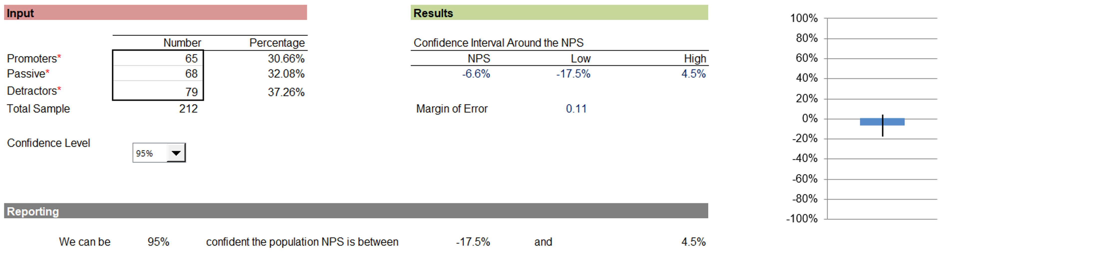
Figure 1: Example of an NPS confidence interval (from the revised MeasuringU NPS Calculator).
2. How to Statistically Compare Net Promoter Scores
Once you construct confidence intervals with an adjusted-Wald method, all you need is algebra to get from a formula for the margin of error to a test of significance, assuming you know the numbers of promoters, passives, and detractors for both sets of NPS data.
In our first article on hypothesis testing for the NPS, we applied the new adjusted-Wald test of significance to compare the GoToMeeting and WebEx data and found a marginally significant difference (Z = 1.815, p = .07). We also conducted a t-test with trinomial means (−1: detractor, 0: passive, +1: promoter) and arrived at the same conclusion (t(65) = 1.86, p = .07). A randomization test on the same data (similar to the bootstrapping we did when comparing confidence intervals) led to the same conclusion but for a slightly higher value for p (.085). We also demonstrated how to construct a confidence interval around the difference using the standard error from the adjusted-Wald Z-test.
Our second article on significance testing broadened our investigation from the first significance testing article. We conducted tests of significance (adjusted-Wald, trinomial means, randomization test) on nine pairs of real-world NPS datasets from our 2020 biennial survey of selected business and consumer software. The pairs had a range of sample sizes and effect sizes (magnitude of differences in the NPS). We found that the adjusted-Wald method worked as well as standard analysis of NPS trinomial means. Both methods had better performance than a randomization test, especially when sample sizes and the NPS differences were small. Based on these results, we recommended that UX researchers who need to conduct a test of significance on pairs of NPS scores use the adjusted-Wald method, especially when used in conjunction with adjusted-Wald confidence intervals.
Figure 2 shows the comparison of the NPS for two products (A: 42.1% and B: 6.4%). The scores are significantly different (p = .001), and the 95% confidence interval around the difference ranges from 14.4% to 54.9%.
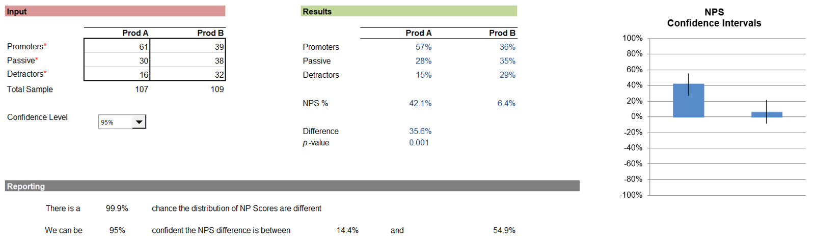
Figure 2: Example of comparison of two sets of NPS data (from the revised MeasuringU NPS Calculator).
We followed that up with an article on how to compare the NPS with a predetermined benchmark. The statistical methods for testing against benchmarks are similar to comparing two NPS, but there are some differences. Most important, because you care only about beating the benchmark, you should use a one-tailed test instead of the more standard two-tailed test, and there is only one variance to estimate because the benchmark is a fixed value.
Figure 3 shows the results of a benchmark comparison where the observed NPS was 42.1% and the benchmark was 20%. The difference of 22.1% is statistically significant (p = .002), and a 95% confidence interval around the difference ranged from 9.3 to 32.5%.
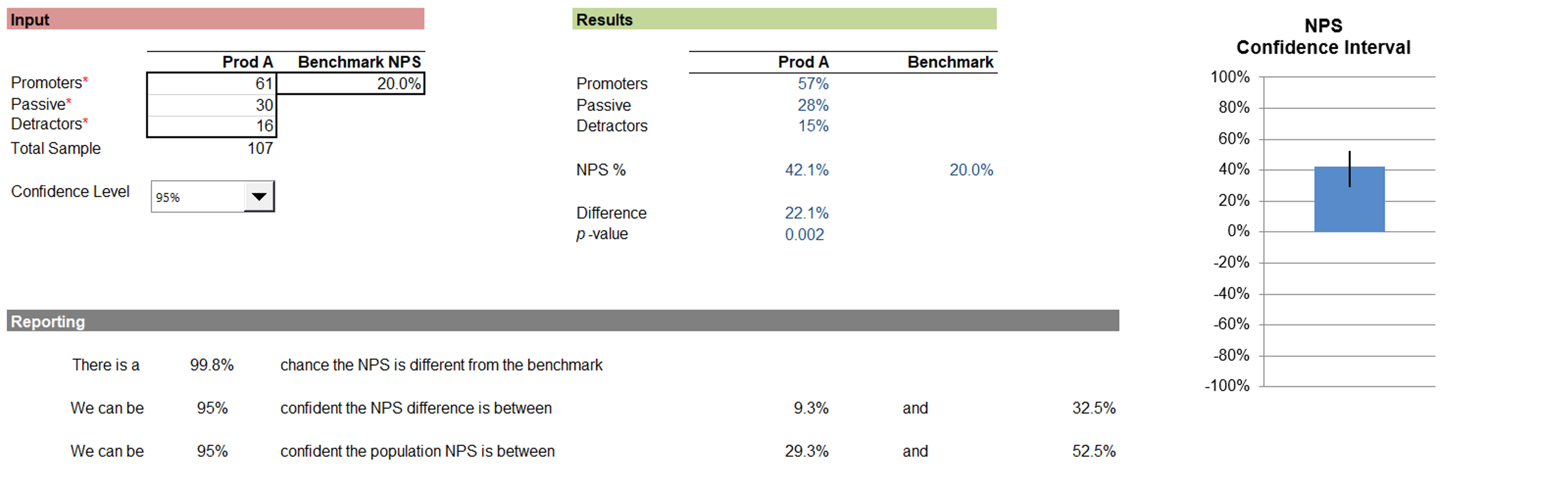
Figure 3: Example of comparison of an NPS with a benchmark (from the revised MeasuringU NPS Calculator).
3. How to Estimate Sample Size Requirements for NPS Analyses
Sample size estimation is a critical step in research planning. Starting with the formulas developed for adjusted-Wald confidence intervals around the NPS and significance testing of the NPS, algebraic manipulation to solve for n leads to methods for sample size estimation.
For confidence intervals, the basic sample size estimation formula is
n = s2Z2/d2 − 3
In the formula, Z is a Z-score whose value is determined by the desired level of confidence. (Common choices are 1.96 for 95% confidence or 1.645 for 90% confidence.) d is the size of the margin of error that reflects your desired precision of measurement (the margin of error). The remaining ingredient is s2, an estimate of measurement variance.
A simple way to estimate variance is to set s2 = 1 (maximum possible variance), but because this method is very conservative (estimating a larger sample size than needed), we don’t recommend it. If you don’t have any data from a previous NPS study, set s2 = .75, where .75 is based on an analysis of 18 real-world sets of NPS data to estimate maximum realistic variance for NPS confidence intervals. You’ll get the most accurate estimate of s2 (and the most accurate sample size estimate) when you have data from a previous study.
If you have data from a previous study, we recommend the maximum accuracy method; otherwise, use the maximum realistic variance method (for which we have a sample size lookup table at the end of this article).
When you compare two NPS, the basic sample size formula is the same (n = s2Z2/d2 − 3), but there are additional complexities to consider when conducting statistical hypothesis testing. Of especial importance is that the value of Z is the sum of two Z scores, one to control Type I errors and the other to control Type II errors (see our article on what can go wrong in statistical hypothesis testing). Additionally, the maximum possible variance is s2 = 2, and the maximum realistic variance is s2 = 1.34. Finally, the resulting sample size estimate is for one group (so the total sample size for two groups will be 2n). As always, when you have previous data for the products you’re comparing, you can get the most accurate estimate of s2.
If you have data from a previous study, we recommend the maximum accuracy method; otherwise, use the maximum realistic variance method (a sample size lookup table for this method is in this article).
For example, suppose we have data from two previous NPS studies that we want to compare. Figure 4 illustrates sample size estimation for comparing those products where the power is 80%, confidence is 90%, and the study can detect differences as small as 20%. The recommended estimate is 205 participants per group (total n = 410).
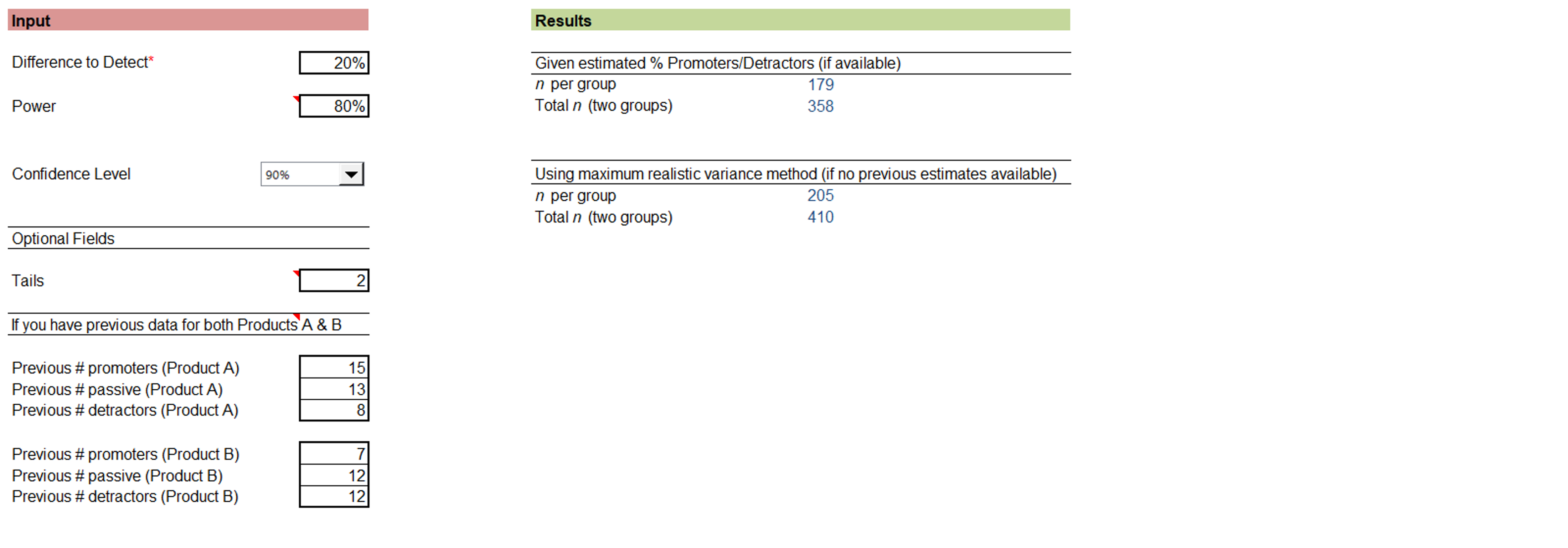
Figure 4: Example of NPS sample size estimation (from the revised MeasuringU NPS Calculator).
For the last article of our NPS series, we completed the set of common analyses with a sample size estimation method that takes special consideration for testing against a benchmark (e.g., testing against a fixed value using a one-tailed instead of a two-tailed test). The basic formula is
n = s2Z2/d2 − 3
The components in this formula are the same as those used to estimate sample sizes for comparing two NPS, including three ways to estimate the variance (s2). For the simplest method assuming maximum variance, s2 = 1; for the maximum realistic variance method, s2 = .67; and for the maximum accuracy method s2 is estimated from previous data. Z is the sum of the Z-scores for the designated levels of confidence (control of the Type I error) and power (control of the Type II error).
We never recommend using the simplest method. Estimation is most accurate when you know the variance from previous data. When there are no data, we recommend the maximum realistic variance method. The article includes a sample size lookup table based on the maximum realistic variance method.