 In math class, we spend a lot of time learning fractions because they are so important in everyday life (e.g., budgeting, purchasing at the grocery store). Fractions are also used extensively in UX research (e.g., the fundamental completion rate is a fraction), typically expressed as percentages or proportions. Unfortunately, fractions are also hard to learn, and as it turns out, they are not the easiest to statistically analyze.
We’ve previously written about how to compare two proportions with the N−1 two-proportion test. This is the correct method to use when the proportions being tested are from two independent groups (e.g., comparing the proportion of online banking users who are under 40 years of age with those who are 40 or older).
But the N−1 two-proportion test is not the correct method when the proportions tested are from the same group of people (e.g., in a within-subjects design comparing the percentage of participants who would be willing to use online banking with the percentage of the same participants who would be willing to use an ATM).
For comparison of dependent proportions, the correct method is the McNemar exact test. See the decision tree in Figure 1 for binary data (measured as 0 or 1 and reported as proportions or percentages). As shown in the figure, follow Y (Yes) at the first branch to compare two proportions, then N (No) because the users are the same in each group, then N (No) for the comparison of two groups.

In this article, we describe how the McNemar exact test works and provide several examples of its use.
How the McNemar Exact Test Works
The test is named for Quinn McNemar, who published it in 1947. His insight was when comparing dependent proportions, the focus needs to be on comparison of discordant rather than concordant proportions.
For example, Table 1 shows the four different possible outcomes for passing or failing a task with Design A or Design B. The concordant proportions are “a” (when participants succeed with both designs) and “d” (when participants fail with both designs). Cases when the user experience is the same with both designs don’t discriminate between the designs, so they are uninformative.
| B Pass | B Fail | Total | |
|---|---|---|---|
| A Pass | a | b | m |
| A Fail | c | d | n |
| Total | r | s | N |
Table 1: Nomenclature for the McNemar exact test.
The discordant proportions are b (when participants succeed with Design A but fail with Design B) and c (when participants fail with Design A but succeed with Design B). These cases are very informative. If the “b” and “c” proportions are about equal, then there’s no evidence that one design is better than the other. If, however, “b” is significantly greater than “c,” then Design A is better, and conversely, if “c” is significantly greater than “b,” then Design B is better.
Note that you can’t set up this table from summary data (just knowing the number of participants who passed and failed with the two designs). You must know the outcomes for each individual to determine the discordant proportions.
One way to get the significance level (p-value) for this comparison is to conduct a sign test (i.e., a nonparametric binomial test) against the null hypothesis that the true proportions for “b” and “c” are the same—50%. The sign test uses the binomial probability formula:
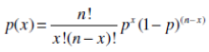
where:
x is the number of positive or negative discordant pairs (cell “b” or “c,” typically use whichever is smaller)
n is the total number of discordant pairs
p = .50 (this is the null hypothesis for the proportion, not to be confused with the significance level that statisticians also designate with the letter “p”)
You could use the exact probabilities generated by the binomial probability formula, but in practice, it’s better to use a technique called “mid-probability” (also referred to as “smoothing” or “continuity correction”), which is less conservative and works well when sample sizes are large or small.
Using the McNemar Exact Test
Here are some examples using the McNemar exact test using the mid-probability p-value.
Example 1: Completion Rates (Small Sample)
Fifteen users attempted the same task on two different designs. The completion rate on Design A was 87% and on Design B was 53%, a fairly large difference of 34%. Table 2 shows how each user performed, with 0s representing failed task attempts and 1s for passing attempts, and Table 3 shows the counts for concordant and discordant responses.
| Participant | Design A | Design B |
|---|---|---|
| 1 | 1 | 0 |
| 2 | 1 | 1 |
| 3 | 1 | 1 |
| 4 | 1 | 0 |
| 5 | 1 | 0 |
| 6 | 1 | 1 |
| 7 | 1 | 1 |
| 8 | 0 | 1 |
| 9 | 1 | 0 |
| 10 | 1 | 1 |
| 11 | 0 | 0 |
| 12 | 1 | 1 |
| 13 | 1 | 0 |
| 14 | 1 | 1 |
| 15 | 1 | 0 |
| Success Rate | 87% | 53% |
Table 2: Successes and failures for 15 participants for task completion with two designs.
| Design B Pass | Design B Fail | Total | |
|---|---|---|---|
| Design A Pass | 7 (a) | 6 (b) | 13 (m) |
| Design A Fail | 1 (c) | 1 (d) | 2 (n) |
| Total | 8 (r) | 7 (s) | 15 (N) |
Table 3: Concordant and discordant responses for 15 participants completing tasks with two designs.
So, we have eight concordant pairs that we don’t care about (a + d), six passing with Design A but failing with Design B (b), and one passing with Design B but failing with Design A (c). On its face, this looks like participants were more successful with Design A (87% higher than 53% for Design B), but is it significantly higher?
To assess the statistical significance of this result, we need to compute its cumulative binomial probability. The simplest way to do this is to focus on the smaller of the discordant cells, computing the probabilities of getting the values from 0 to the observed value of 1:
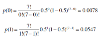
The value of the mid-probability for a two-tailed McNemar test is the sum of the probabilities for the number of discordant pairs in the cell of interest (c in this example) plus half of the probability of the observed number, and multiplying that number by two, for this example, (.0078 + .0547/2)(2) = .0352(2) = .0704.
The probability of seeing one out of seven participants perform better on Design A than B if there really is no difference is about .07. Whether that is statistically significant depends on the chosen alpha criterion. Using a common industrial criterion, we find the difference is statistically significant with p < .10.
Example 2: Comparison of Top-Box Scores (Large Sample)
Given how tedious it is to work through the McNemar exact test procedure by hand for a small sample, it’s good to know that calculators can take care of the computations, which we demonstrate in this example.
In a study of rating scale formats, 256 respondents completed an online survey in which they used two different versions of the UX-Lite questionnaire that differed in the numbers assigned to their response options (Standard: 1 to 5; Alternate: −2 to +2). Table 4 shows the patterns of top-box scores for these dependent ratings, where a top-box rating was assigned a score of 1 and all other ratings a score of 0.
| Alternate 1 | Alternate 0 | Total | |
|---|---|---|---|
| Standard 1 | 123 | 18 | 141 |
| Standard 0 | 22 | 93 | 115 |
| Total | 145 | 111 | 256 |
Table 4: Concordant and discordant responses for the UX-Lite scale format study.
When the sample size is large, the best way to build this table is by cross-tabbing the two variables of interest (a procedure called pivot tables in Excel).
This information is all you need to use a McNemar exact test calculator to determine the p-value for statistical significance. You could search for a calculator online, but be cautious because few online calculators offer the option for a mid-p binomial test of the results, and even when they do, they may provide questionable statistical guidance for interpreting the result.
We prefer using the calculator that is part of the MeasuringU Usability Statistics Package Expanded, as shown in Figure 2. As expected, given how little difference there was in top-box scores for the two types of discordant pairs (18 vs. 22 out of 256 respondents, only about a 1.5% difference), the p-value for the test was not statistically significant (p = .53).

Confidence Intervals for McNemar Exact Tests
Establishing whether a comparison of percentages for matched pairs is statistically significant is only one step in the process of assessing practical significance. To do that, we need to compute a confidence interval around the observed difference.
Just as there are variations of the McNemar exact test, there are also different ways to compute associated confidence intervals. We prefer the Agresti and Min (2005 [PDF]) adjusted-Wald interval modified for differences in the kinds of matched pairs assessed with the McNemar exact test.
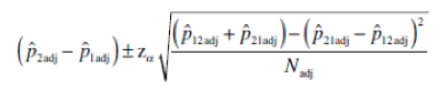
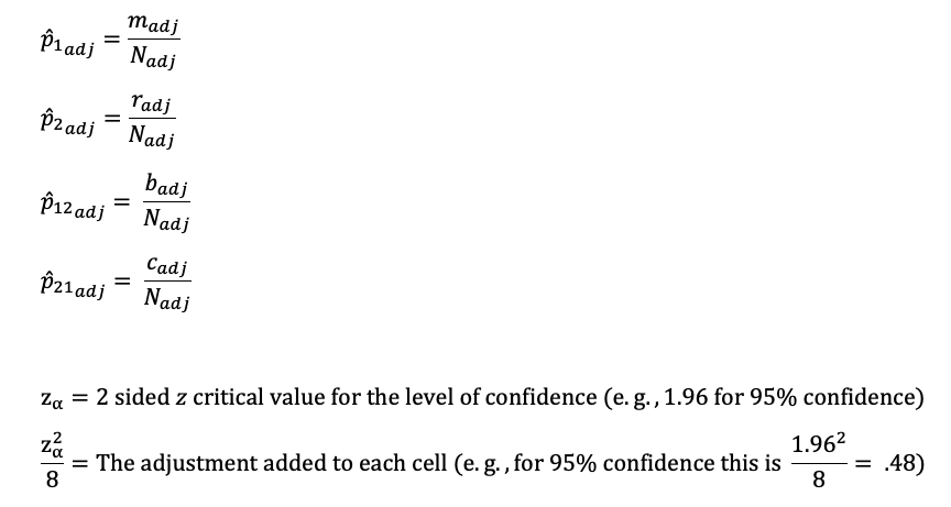
When applied to a 2 × 2 table for a within-subjects setup (as in the McNemar exact test), the adjustment is to add 1/8th of a squared critical value from the normal (z) distribution for the specified level of confidence to each cell in the 2 × 2 table. The resulting formula (where “adj” means the adjustment has been added to cells a, b, c, and d) is:
Using the nomenclature from Table 1:
Example 1: Completion Rates (Small Sample)
Continuing with our first example, we’ll show how to compute the 95% confidence interval by hand (simplifying a bit by using .5 for the adjustment instead of .48), using the adjusted values in Table 5.
| Design B Pass | Design B Fail | Total | |
|---|---|---|---|
| Design A Pass | 7.5 | 6.5 | 14 |
| Design A Fail | 1.5 | 1.5 | 3 |
| Total | 9 | 8 | 17 |
Table 5: Adjusted concordant and discordant responses for the successful task completion example.
Putting these adjusted values into the confidence interval formula, we get:
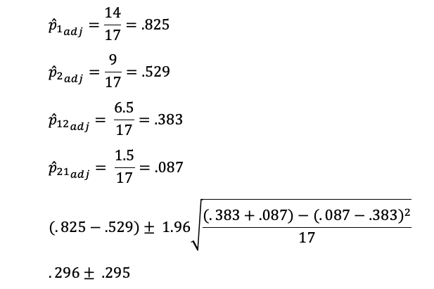
The 95% confidence interval around the 34% difference in completion rates between designs is 0.1% to 59.1%. The confidence interval does not include 0, so the difference is statistically significant. Because the lower limit of the confidence interval is just 0.1%, it’s plausible that the difference could actually be that small, so even though the result was statistically significant, its practical significance has not been firmly established. The magnitude of the observed difference, however, is an indicator that Design A is probably the better design.
Example 2: Comparison of Top-Box Scores (Large Sample)
A good calculator for the McNemar exact test should also provide a confidence interval with the desired confidence level in its output, but very few do.
Referring to Figure 2 (output from the MeasuringU® Usability Statistics Package Expanded), the 95% confidence interval around the difference ranged from −3.1 to 6.0 around the observed difference of about 1.5%. In this example, the outcome indicates neither a statistically nor practically significant result.
Summary
The McNemar exact test is appropriate for evaluating the statistical significance of the difference between two dependent proportions collected in a within-subjects study.
The McNemar exact test focuses on the difference in discordant proportions. When a pair of binary variables have different outcomes—e.g., (0, 1) or (1, 0)—they are discordant. When the outcomes are the same—e.g., (0, 0) or (1, 1)—they are concordant. Because concordant outcomes are the same in both conditions, they are not informative for discriminating between the conditions. By analyzing discordant proportions, the McNemar exact test can discriminate between the within-subjects conditions of interest.
One way to determine the statistical significance of a McNemar exact test is to run a sign test. A sign test is a binomial test in which the null hypothesis is that the proportions of the two different types of discordant proportions are equal. When conducting a sign test, it’s better to use mid-probabilities than exact probabilities for p-values.
Use a modified adjusted-Wald confidence interval to assess the precision of the estimated difference in discordant proportions. This is the method published by Agresti and Min (2005), where the adjustment is to add 1/8th of a squared critical z-value for the specified level of confidence to each cell in the 2 × 2 summary of the concordant and discordant pairs (e.g., about .5 for 95% confidence).