 Microsoft Word is a widely used word processing program, part of the Microsoft Office suite of programs.
While its dominance has been challenged recently by Google Docs, Word still leads on the features list, providing many features that Google’s offering lacks. But adding features can also add to bloat, making common tasks harder as users have to navigate ever-expanding menus and ribbons. Has Word’s ease-of-use suffered over the past few years?
The System Usability Scale (SUS) is one of the more common ways to measure the perceived ease of use of software. We’ve been tracking Microsoft Word’s SUS for over a decade.
Figure 1 shows that Word had a SUS score of 74.7 in our 2020 report (data collected in late 2019), about a 7.5-point drop from our 2017 report.
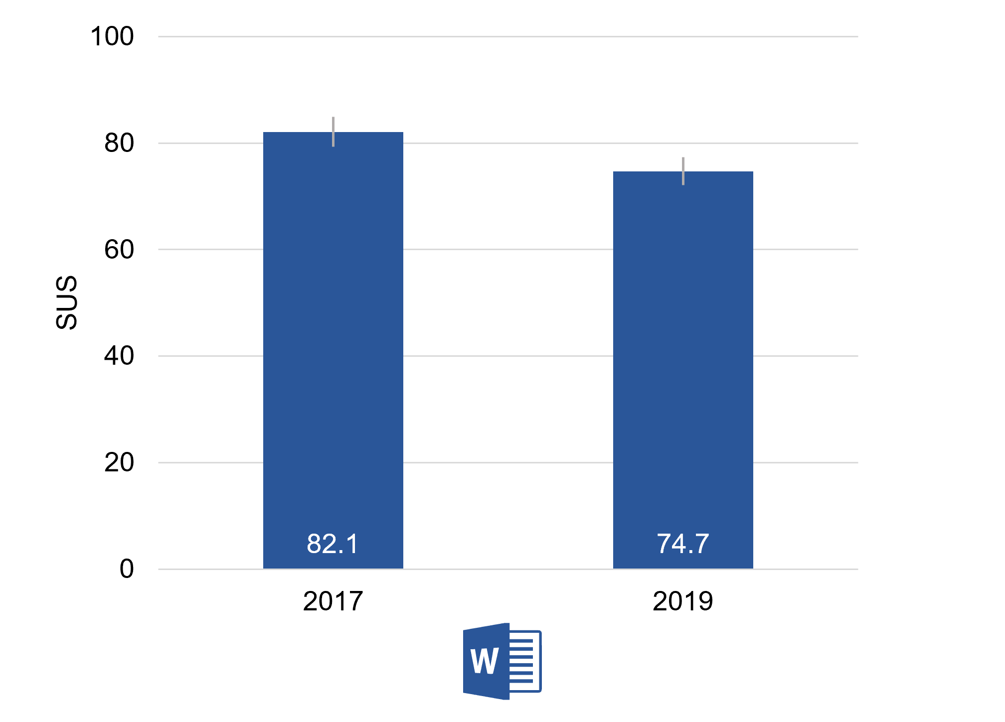
That drop in SUS means is statistically significant (t(272) = 3.8, p =.0002), but what sample size did we need to find these statistical differences? The sample sizes were 170 and 111 in the 2017 and 2020 datasets respectively. (It’s easy to find Word users so our cost per sample is low.)
But do you always need a sample size over 100? What if the cost for each additional sample is $20 or $200? In fact, any sample size larger or smaller than what you need is potentially wasteful of resources. When can you use a small sample size, and when should you plan on a very large sample size to find statistical significance?
The answer to those questions depends on several different factors, starting with the expected type of analysis.
In previous articles, we’ve covered how to estimate sample sizes for SUS confidence intervals (constructing the plausible range of values around the mean for a sample of data) and benchmark tests (comparing a single sample of SUS scores against a set benchmark like the historical mean of 68 or a more aspirational target of 80, an A− on the Sauro-Lewis curved grading scale for the SUS).
In this article, we discuss the additional considerations required to compare two mean SUS scores.
What Drives Sample Size Requirements for Comparison Tests?
To compute a sample size requirement, you always need an estimate of the variability of the measure (standard deviation), a judgment of the required precision of measurement, and a judgment of the desired confidence level. In fact, these are all you need to compute the sample size requirement for studies in which you only plan to compute a confidence interval around a mean.
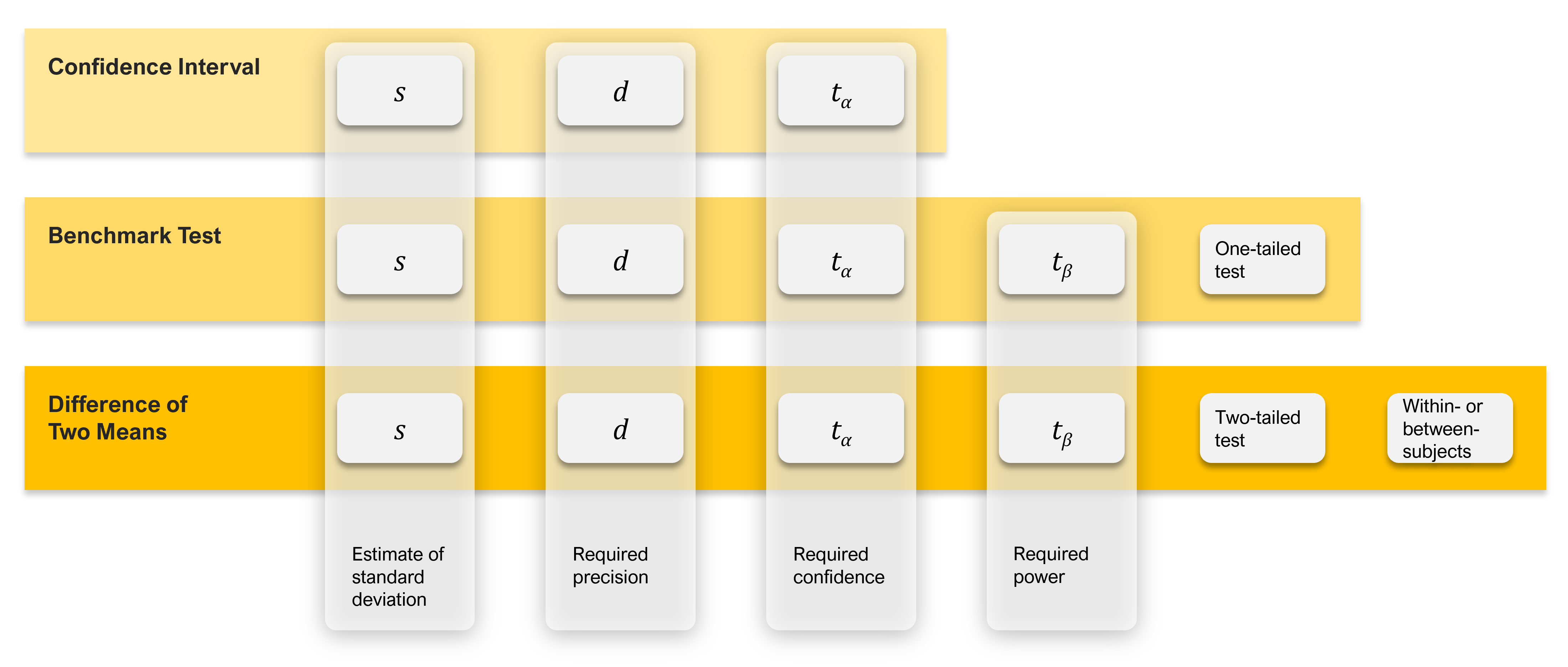
As shown in Figure 2, you need to know six things to compute the sample size when comparing two means. The first three are the same elements required to compute the sample size for a confidence interval:
- An estimate of the SUS standard deviation: s
- The required level of precision (using SUS points or percentages): d
- The level of confidence (typically 90% or 95%): tɑ
For a comprehensive discussion of these three elements, see our previous confidence interval article.
Sample size estimation for benchmark and comparison studies also requires two additional considerations:
- The power of the test (typically 80%): tβ
- The distribution of the rejection region (one-tailed for benchmark tests, two-tailed for means)
And the comparison of two means has one more consideration:
- Within (same people in each sample) or between-subjects study (different people in each sample)
Figure 2 illustrates how the number of sample size drivers increases and changes from confidence intervals (the simplest with three drivers) to benchmark testing (five drivers) to tests of two means (six drivers).
Quick Recap of Power and Tails (Rejection Regions)
The power of a test refers to its capability to detect a specified minimum difference between means (i.e., to control the likelihood of a Type II error). The number of tails refers to the distribution of the rejection region for the statistical test. In the vast majority of cases, comparisons of two SUS means should use a two-tailed test. For more details on these topics, see the previous article on SUS benchmark testing.
Sample Size Formulas for Within- and Between-Subjects Studies
In a within-subjects study, you compare the means of scores that are paired because they came from the same person (assuming proper counterbalancing of the order of presentation). In a between-subjects study, you compare the means of scores that came from different (independent) groups of participants. Each experimental design has its strengths and weaknesses. The formulas for sample size estimation are different for the two experimental designs.
Within-Subjects
The sample size formula for a within-subjects study is the same as the one used for benchmark tests:
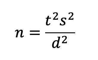
where s is the standard deviation (s2 is the variance), t is the t-value for the desired level of confidence AND power, and d is the target for the critical difference (the smallest difference in means that you need to be able to detect).
As in benchmark testing, t in the formula is the sum of two t-values, one for ɑ (related to confidence, two-sided for comparison of means) and one for β (related to power, always one-sided). For a 90% confidence level and 80% power this works out to be about 1.645 + 0.842 = 2.5.
One way to think of including power in sample size estimation is as an insurance policy. You purchase the policy by increasing your sample size, improving your likelihood of finding statistically significant results if the standard deviation is a little higher than expected or the observed value of d is a bit lower.
Between-Subjects
The sample size formula for a between-subjects study is the basic equation multiplied by 2. (For details on its derivation, see Chapter 6 in Quantifying the User Experience.) Note that this formula is for the sample size of one independent group, so if you are comparing two means, the total sample size will be twice this number.
Sample Size Tables
Table 1 shows the sample sizes required for two levels of confidence (90% and 95%), one level of power (80%), assumption of two-tailed testing, and various levels of d from 1 to 15, using our best estimate of the typical standard deviation of the SUS (17.7) for within- and between-subjects studies.
| d | Within; 90% | Within; 95% | Between; 90% | Between; 95% | |
|---|---|---|---|---|---|
| 15 | 11 | 13 | 38 | 46 | |
| 10 | 21 | 27 | 80 | 102 | |
| 7.5 | 36 | 46 | 140 | 178 | |
| 5 | 80 | 101 | 312 | 396 | |
| 2.5 | 312 | 396 | 1,242 | 1,576 | |
| 2 | 486 | 617 | 1,940 | 2,462 | |
| 1 | 1,939 | 2,461 | 7,750 | 9,838 |
Table 1: Sample size requirements for various critical differences (two-tailed, 80% power, s = 17.7. Between-subjects cells are the total sample size for a two-group study).
For example, if you want to be able to detect mean differences of 15 with 90% confidence and 80% power in a within-subjects study, you’d need a sample size of 11. For the same requirements in a between-subjects study, you’d need a total sample size of 38 (19 per group).
At the other end of the table, for 95% confidence, 80% power, and a critical difference of 1 in a within-subjects study, you’d need a sample size of 2,461. For the same requirements in a between-subjects study, you’d need a total sample size of 9,838 (4,919 per group).
In this table, there’s a sort of Goldilocks zone (highlighted in green) with reasonably small requirements for the critical difference (d from 2.5 to 5 for within-subjects studies; 5 for between-subjects studies), which have reasonably attainable sample size requirements (n from 80 to 396).
Returning to the example we started with, what sample size would we need for a between-subjects comparison of SUS means to find a difference as small as 7.5 points with 95% confidence and 80% power? Using Table 1, we would plan on a sample size of 178 (about 89 in each group). If we needed to reliably detect differences as small as 5, we’d need a sample size of 396 (about 198 in each group).
The table also shows how sample size estimates balance statistics and logistics. The math for a high level of discrimination between SUS means may indicate aiming for a sample size of 2,000 or more, but the feasibility (cost and time) of obtaining that many participants might be prohibitive, even in a retrospective survey or unmoderated usability study where the cost of each sample is fairly low.
What about the Different Estimates for the Standard Deviation of SUS?
As documented in A Practical Guide to the System Usability Scale, estimates of the standard deviation of the SUS from different sources ranged from 16.8 to 22.5. A standard deviation of 17.7 is typical, but what if your standard deviation is larger than that?
For example, suppose your estimate is 20. Because this estimate is larger than the 17.7 used to build Table 1, when all other things are the same (e.g., confidence, power, and critical differences) you’ll need larger sample sizes, as shown in Table 2.
| d | Within; 90% | Within; 95% | Between; 90% | Between; 95% | |
|---|---|---|---|---|---|
| 15 | 13 | 16 | 46 | 58 | |
| 10 | 27 | 34 | 102 | 128 | |
| 7.5 | 46 | 58 | 178 | 226 | |
| 5 | 101 | 128 | 398 | 506 | |
| 2.5 | 398 | 505 | 1,586 | 2,012 | |
| 2 | 620 | 787 | 2,476 | 3,142 | |
| 1 | 2,475 | 3,142 | 9,894 | 12,562 |
Table 2: Sample size requirements for various critical differences (two-tailed, 80% power, s = 20. Between-subjects cells are the total sample size for a two-group study).
If your SUS data has a standard deviation close to 17.7, use Table 1. If it’s closer to 20, use Table 2. If it’s in between, then you can interpolate the values in Tables 1 and 2 to get an idea about the approximate sample size. If you need a more precise estimate, see the following technical note.
Technical Note: If you’re working with SUS data that has a very different standard deviation from 17.7 or 20, you can do a quick computation to adjust the values in these tables. The first step is to compute a multiplier by dividing the new target variance (s2) by the variance used to create the table. Then multiply the tabled value of n by the multiplier and round it off to get the revised estimate. For example, if the target standard deviation (s) is 19.1, the target variability (s2) is 364.81. The variability from Table 2 is 400 (202), making the multiplier .912 (364.81/400). To use this multiplier to adjust the sample size of 398 for 90% confidence and critical difference of 2.5 shown in Table 2 for a within-subjects design, multiply 398 by .912 and then round it off to 363. For a between-subjects design with the same requirements, multiply 1586 by .912 and round it off to 1,446 (723 per group).
Summary and Takeaways
What sample size do you need when comparing two sets of SUS scores? To answer that question, you need several types of information, some common to all sample size estimation (confidence level to establish control of Type I errors, standard deviation, and margin of error or critical difference), others unique to statistical hypothesis testing (one- vs. two-tailed testing, setting a level of power to control Type II errors), and for comparison of means, whether the experimental design will be within- or between-subjects.
We provided two tables based on a typical standard deviation for the SUS in retrospective UX studies (s = 17.7) and a more conservative standard deviation (s = 20), with values for between- and within-subjects designs, 90% and 95% confidence, and power set to 80%.
For UX researchers working in contexts where the typical standard deviation of the SUS might be different, we also provided a simple way to increase or decrease the tabled sample sizes for larger or smaller standard deviations.