
The two-sample t-test is one of the most widely used statistical tests, assessing whether mean differences between two samples are statistically significant. It can be used to compare two samples of many UX metrics, such as SUS scores, SEQ scores, and task times.
The t-test, like most statistical tests, has certain requirements (assumptions) for its use.
While it’s easy to conduct a two-sample t-test using readily available online calculators and software packages (including Excel, R, and SPSS), it can be hard to remember what the assumptions are and what risks you run by not meeting those assumptions.
In teaching statistical tests to UX researchers over the last decade, we’ve found that the possible violation of assumptions is a common concern about using t-tests. In some cases, researchers report challenges from stakeholders or colleagues to justify their use of t-tests due to concerns about meeting assumptions.
One way to respond to this criticism is to cite the large volume of research that shows the t-test to be very robust against violations of its assumptions. Figure 1 shows the assumptions behind the two-sample t-test.
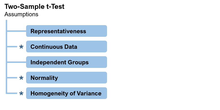
Figure 1: Assumptions of the two-sample t-test (* = test is robust against violations of this assumption).
Unlike the other three assumptions, the assumptions of representativeness and independence have nothing to do with the underlying distribution. These are logical assumptions made whenever you use any method to compare means to generalize results from samples to populations.
For the assumption of continuous data, even if the data themselves are not continuous (e.g., discrete responses to rating scales), the mean becomes more and more continuous as the sample size increases. Violation of this assumption does not prevent the t-test from working.
The assumption of normality is not an assumption that the underlying distribution is normal but rather that the distribution of sample means will be normal. For most distributions, this will be the case due to the central limit theorem—even for fairly small sample sizes. For some types of data, you can transform the data to enhance normality (e.g., logarithmic transformation of task times).
Finally, research has shown that the variance between the two groups needs to be great for the violation of the assumption of homogeneity to affect results. When that happens, adjusting the degrees of freedom can compensate for the violation.
Another strategy is to analyze the data with a nonparametric test to see if you get the same result. There are different types of nonparametric tests, including rank tests and resampling tests. Of these, the approach that makes the fewest assumptions about underlying distributions is the randomization test, a type of distribution-free nonparametric test.
We’re not advocating that researchers abandon the t-test when analyzing typical UX data. In our practice, we intend to keep using the t-test as a statistical workhorse, making adjustments to degrees of freedom (when variances are radically different) and using logarithmic transformations (for time data) as needed. (For details, see Quantifying the User Experience, 2nd ed.)
There could be times, however, when UX researchers may need to use a distribution-free method to compare two independent means: a client’s request, a response to criticism for failing to meet the assumptions of the t-test, or to double-check the results of t-tests when analyzing data that may have radically violated multiple assumptions of the t-test.
In this article, we describe how randomization tests work and demonstrate how to run one using the open-source R programming language.
What Is a Randomization Test?
A modern randomization test uses software to shuffle data before computing values (for example, mean and median differences) and to compare the results after shuffling to the original data. Repeat the process thousands of times to generate a proportion similar to the p-value you get in a t-test. But randomization tests predate computers. To understand what a randomization test is, it helps to know where it came from.
R. A. Fisher was the first to describe a randomization test, in his 1935 book The Design of Experiments (in which he also described the use of Greco-Latin squares in experimental design). The second chapter included his famous lady tasting tea experiment, based on an actual event. In this experiment, he computed how likely it would be for someone randomly presented with eight cups of tea to guess which four had milk added to tea (the other four had tea added to milk). Because there were 70 unique combinations in which the eight cups of tea could be presented, the likelihood of someone guessing all of them correctly would be 1/70, or .014. Thus, if someone did provide a set of correct judgments (as reportedly occurred), it would not be likely to happen by chance.
In Fisher’s tea experiment, it was possible to enumerate all possible combinations, but for large experiments that approach is unwieldy. The workaround is to shuffle a set of data many times (usually 5,000–10,000 iterations), and to compare after each shuffle the randomized result with the result obtained from the experimental data.
Comparing Two Means with R
How to Conduct a Randomization Test
Here is the general process for computing a randomization test to compare the means from two samples:
- Compute two means. Compute the mean of the two samples (original data) just as you would in a two-sample t-test.
- Find the mean difference. Compute the difference between means.
- Combine. Combine both samples into one group of data.
- Shuffle. Shuffle the order of the combined group.
- Select new samples. Randomly sample the same number of values for two new samples as you did in the original data. For example, if your original sample had 10 values in the first condition and 13 values in the second, select the first 10 values for sample 1 and the next 13 for sample 2.
- Compute two new means. Compute the means of the two new samples.
- Find the new mean difference. Find the new difference between means.
- Compare mean differences. If the absolute value of the difference after shuffling is more than or equal to the original mean difference, record 1 for this iteration; if not, give it 0.
- Iterate. Repeat 1,000+ times (we usually use 10,000 iterations).
- Compute p. The percentage of 1s is the p-value for the test. If the observed mean difference is unlikely to have happened by chance, this percentage will be small.
Below, we present two examples of randomization tests.
If you’re interested in trying these examples yourself, see the appendix at the end of this article for instructions on how to get and install R and how to download the R script and data files used in the examples.
Example 1: Comparing Completion Times
The first example is from pp. 70–71 of Quantifying the User Experience (2nd ed). Twenty users were asked to add a contact to a CRM application, with 11 using an old design and 9 using a new design, so the total sample size was 20, with n1 = 11 and n2 = 9 (times are in seconds).
To illustrate how shuffling works, Table 1 shows the observed data and five sample runs through an R function we developed to run randomization tests (for details, see the appendix). For each sample run, the data were shuffled, then the mean of the second 9 task times was subtracted from the mean of the first 11. For the randomized runs, the absolute mean differences ranged from 0.3 to 5.5—all much lower than the observed difference of 18.9. This suggests that the observed difference of 18.9 is probably not due to chance, but to prove it, we need more iterations.
| Condition | Original | Run 1 | Run 2 | Run 3 | Run 4 | Run 5 |
|---|---|---|---|---|---|---|
| Old | 18 | 10 | 20 | 20 | 44 | 77 |
| Old | 44 | 9 | 21 | 9 | 78 | 2 |
| Old | 35 | 12 | 30 | 22 | 35 | 12 |
| Old | 78 | 22 | 2 | 44 | 21 | 10 |
| Old | 38 | 44 | 77 | 12 | 40 | 35 |
| Old | 18 | 30 | 18 | 2 | 9 | 20 |
| Old | 16 | 16 | 10 | 78 | 30 | 35 |
| Old | 22 | 35 | 35 | 38 | 2 | 38 |
| Old | 40 | 18 | 22 | 21 | 18 | 16 |
| Old | 77 | 38 | 12 | 35 | 18 | 38 |
| Old | 20 | 77 | 38 | 18 | 10 | 40 |
| New | 12 | 35 | 9 | 35 | 35 | 5 |
| New | 35 | 78 | 35 | 30 | 16 | 9 |
| New | 21 | 20 | 40 | 38 | 77 | 30 |
| New | 9 | 2 | 5 | 40 | 38 | 44 |
| New | 2 | 21 | 18 | 18 | 20 | 21 |
| New | 10 | 5 | 78 | 77 | 5 | 18 |
| New | 5 | 40 | 38 | 5 | 12 | 22 |
| New | 38 | 18 | 16 | 16 | 22 | 18 |
| New | 30 | 38 | 44 | 10 | 38 | 78 |
| Old Mean | 36.9 | 28.3 | 25.9 | 27.2 | 27.7 | 29.4 |
| New Mean | 18.0 | 28.6 | 31.4 | 29.9 | 29.2 | 27.2 |
| |Difference| | 18.9 | 0.3 | 5.5 | 2.7 | 1.5 | 2.1 |
Table 1: Five sample runs through the resample.u.between function.
A two-sample t-test (two-sided) of the observed data found the difference to be statistically significant (t(16) = 2.33, p = .033). To see how this compares with a randomization test, we ran our R function:
resample.u.between(‘sampletimes.txt’,11,9,10000)
The arguments for the resample.u.between function are the name of the data file, n1, n2, and the number of iterations. Figure 2 (a screenshot of the R console) shows the observed difference of 18.9 and the percentage of 10,000 randomizations in which the mean difference was equal to or greater than 18.9, which was .0355—just a bit higher than the p-value from the t-test. Note that repeated runs of randomization tests will have some variation in the reported percentage, but with 10,000 iterations their variance will be small.
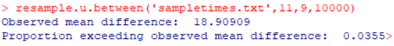
Figure 2: Result of randomization test assessing significance of completion times with old and new CRM designs.
Example 2: Comparing SUS Scores
On pp. 67–68 of Quantifying the User Experience (2nd ed), we computed a two-sample t-test for a set of System Usability Scale (SUS) scores, collected when 23 participants rated their experience attempting a task with two different CRM applications, with 11 using Product A and 12 using Product B. Product A had a mean SUS score of 51.6 (sd = 4.07), and Product B had a mean of 49.6 (sd = 4.63). The resulting t-test indicated the observed difference of 2.0 was not statistically significant (t(21) = 1.1, p = .2835).
Figure 3 shows the result of comparing the data with the randomization test function. The proportion exceeding the observed mean difference was 0.2891—very close to the p-value from the t-test.
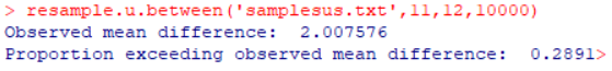
Figure 3: Result of randomization test assessing significance of SUS scores with CRM Products A and B.
Summary and Discussion
Randomization tests use computer functions to randomly shuffle data many times. To evaluate mean differences, after each shuffle, the means computed from the shuffled data are compared with the observed mean difference. The p-value for the randomization test is the percentage of times the absolute value of the shuffled mean difference is equal to or greater than the absolute value of the observed mean.
In two examples, we found close matches between the p-values from two-sample t-tests and randomization tests. Both of our examples used data that violated assumptions of the t-test (Example 1 used time data that violated assumptions of normality; Example 2 used SUS data that violated the assumption of continuous data). So, these results are consistent with research showing the robustness of the t-test against such violations.
We do not generally recommend using randomization tests instead of t-tests for standard UX metrics. However, they could be a valuable tool for UX researchers who need to perform a sanity check (or to address concerns from colleagues) when working with atypical data that radically violates multiple assumptions of the two-sample t-test.
Appendix: Instructions for Downloading R, the R Script, and Data Files
If you’re interested in trying this out for yourself, follow these instructions to download and install R. The appendix also has links to the R script file for the resample.u.between function and the two sample data files.
Getting and Installing R
To run the following script, you’ll have to get and install R. We’ll be demonstrating the command line interface, so all you need is the basic installation. To install R:
- Go to http://www.r-project.org/.
- In the Getting Started section, click the “download R” link. This takes you to a list of CRAN (Comprehensive R Archive Network) mirrors. Each “mirror” is a website from which you can get R. Go down the list to find your country (e.g., USA) and select one of the sites (e.g., http://cran.case.edu/).
- Depending on the type of computer you have, select the appropriate version of R to download (Linux, Mac OS X, or Windows).
- Select “base.” This takes you to the download page for first-time installers.
- Click the “Download R” link, which downloads an executable (.exe) file that you can double-click to complete the installation (follow the on-screen instructions).
- Double-click the R desktop icon to start the R console.
The R Script and Sample Data Files
Use the following links to download the R script we developed for our randomization test and the sample data files. R files are regular text files with an “R” extension. By default, the R console uses the Documents folder on a Windows machine, so R files and data files are easiest to use when you put them in the Documents folder. To open an R file in the console, click File > Source R code … then double-click the desired R file. To use the randomization test function, enter “resample.u.between(‘dataFileName’,n1,n2,iterations)”. The first argument is the name of the data file, n1 is the sample size for the first condition, n2 is the sample size for the second condition, and iterations is the number of times to do the resampling (we usually set this to 10000).