 The UX-Lite® is a relatively new metric, but it is versatile, short, and increasingly popular for UX research. It measures perceived usability and usefulness with just two items.
But if you’re using the UX-Lite to compare products or to see whether you’ve improved over time, what sample size do you need?
Yes, the sample size question we can’t (and shouldn’t) avoid. Fortunately, sample sizes for making comparisons are straightforward and uncontroversial.
In previous articles, we’ve developed sample size tables for studies focused on estimating UX-Lite scores with confidence intervals or comparing them to benchmark values.
The UX-Lite, like the SUS, uses transformed scores that range from 0 to 100, based on responses to its two five-point scales (usability and usefulness). We refer to it as a mini version of the 16-item Technology Acceptance Model (TAM). The UX-Lite predicts the SUS with over 95% accuracy, and like the TAM, it predicts future product usage.
In this article, we cover how to determine appropriate sample sizes for comparing two mean UX-Lite scores.
What Drives Sample Size Requirements for Comparison Tests?
You need to know six things to compute the sample size when comparing two means. The first three are the same elements required to compute the sample size for a confidence interval:
- An estimate of the UX-Lite standard deviation (median of 19.3 with an interquartile range from 16.6 [25th percentile] to 21.3 [75th percentile]): s
- The required level of precision: d
- The level of confidence (typically 90% or 95%): tɑ
For a more detailed discussion of these three elements, see our previous confidence interval article.
Sample size estimation for benchmark and comparison studies requires two additional considerations:
- The power of the test (typically 80%): tβ
- The distribution of the rejection region (one-tailed for benchmark tests, two-tailed for means)
As a quick recap, the power of a test refers to its capability to detect a specified minimum difference between means (i.e., to control the likelihood of a Type II error). The number of tails refers to the distribution of the rejection region for the statistical test. In most cases, comparisons of two means should use a two-tailed test. For more details on these topics, see the previous article on UX-Lite benchmark testing.
The comparison of two means has one more consideration:
- Within- or between-subjects experimental design
In a within-subjects study, you compare the means of scores that are paired because they came from the same person (assuming proper counterbalancing of the order of presentation). In a between-subjects study, you compare the means of scores that came from different (independent) groups of participants. Each experimental design has its strengths and weaknesses, and each has its own formula for sample size estimation.
Figure 1 illustrates how the number of sample size drivers increases and changes from confidence intervals (the simplest with three drivers) to benchmark testing (five drivers) to tests of two means (six drivers).
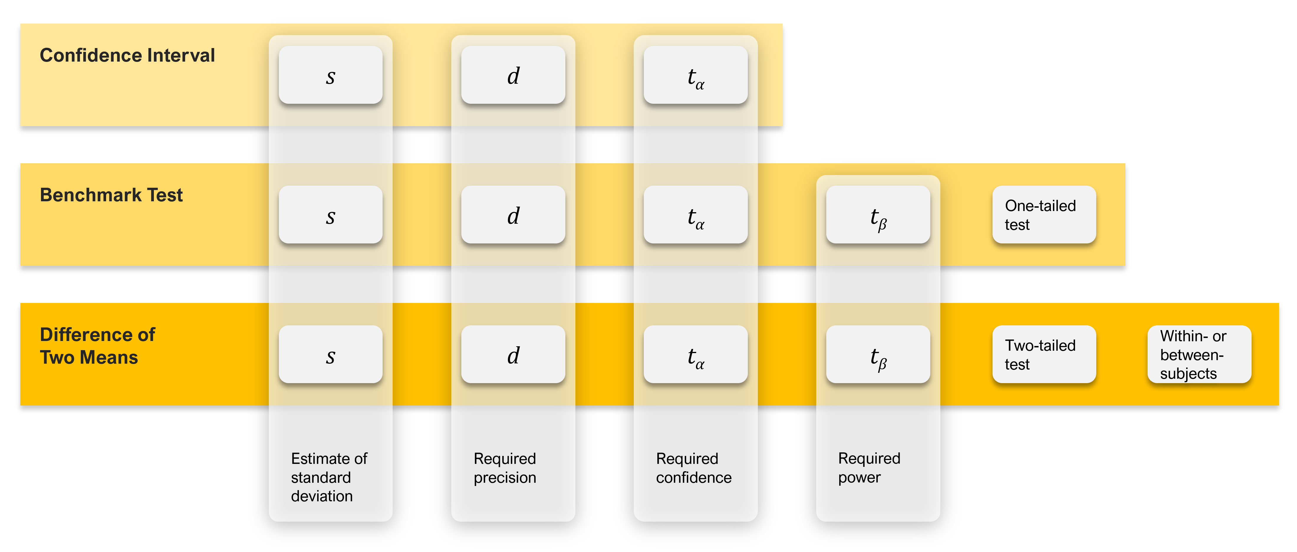
Figure 1: Drivers of sample size estimation for comparing scores.
UX-Lite Sample Sizes for Within-Subjects Comparison of Two Means
The sample size formula for a within-subjects study is the same as the one used for benchmark tests:
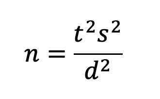
where s is the standard deviation (s2 is the variance), t is the t-value for the desired level of confidence AND power, and d is the target for the critical difference (the smallest difference in means that you need to be able to detect).
As in benchmark testing, t in the formula is the sum of two t-values, one for ɑ (related to confidence, two-sided for comparison of means) and one for β (related to power, always one-sided). For a 90% confidence level and 80% power, this works out to be about 1.645 + 0.842 = 2.5.
One way to think of including power in sample size estimation is as an insurance policy: you purchase the policy by increasing your sample size, improving your likelihood of finding statistically significant results if the standard deviation is a little higher than expected or the observed value of d is a bit lower.
Table 1 shows how variations in these components affect sample size estimates for within-subjects comparisons for the median standard deviation of 19.3 and for the 75th percentile of 21.3. In most cases, using the median standard deviation is reasonable, but when a sufficient sample size is more important than controlling the cost of sampling, it’s better to plan with the higher value.
| d | ||||
| 15 | ||||
| 10 | ||||
| 7.5 | ||||
| 5.0 | ||||
| 2.5 | ||||
| 2.0 | ||||
| 1.0 | ||||
Table 1: Sample size requirements for UX-Lite comparisons within subjects given various standard deviations (s), confidence levels, and critical differences (d), with power set to 80%.
In this table, the “magic range” for the critical difference is from 2.5 to 5, where the sample sizes are reasonably attainable (n from 94 to 572). The table also illustrates the tradeoff between the ability of a test to detect significant differences and the sample size needed to achieve that goal.
For example, if you want to be able to detect mean differences of 15 with 90% confidence and 80% power in a within-subjects study, you’d need a sample size of 12. At the other end of the table, for 95% confidence, 80% power, and a critical difference of 1 in a within-subjects study, you’d need a sample size of 3,563.
UX-Lite Sample Sizes for Between-Subjects Comparison of Two Means
The only change for a between-subjects comparison is to the sample size formula that roughly doubles the sample size for each group and, because there must be two groups, doubles that again. This means that to achieve the same level of sensitivity while keeping everything else equal, the sample size for a between-subjects comparison is about four times the sample size required for a within-subjects comparison. As shown in Table 2, this constrains the “magic range” for a reasonable critical difference to no less than 5, for which the sample sizes for the various combinations of standard deviation and confidence level range from 372 to 572.
| d | ||||
| 15 | ||||
| 10 | ||||
| 7.5 | ||||
| 5.0 | ||||
| 2.5 | ||||
| 2.0 | ||||
| 1.0 | ||||
Table 2: Sample size requirements for UX-Lite comparisons between subjects given various standard deviations (s), confidence levels, and critical differences (d), with power set to 80% and total sample sizes for two independent groups.
Technical Note: What to Do for Different Standard Deviations
If your historical UX-Lite data has a very different standard deviation from 19.3 or 21.3, you can do a quick computation to adjust the values in these tables. The first step is to compute a multiplier by dividing the new target variance (the square of the standard deviation, s2) by the variance used to create the table. Then multiply the tabled value of n by the multiplier and round it to get the revised estimate. To illustrate this, we’ll start with a standard deviation of 19.3 (our typical standard deviation) and show how this works if the target standard deviation (s) is 21.3 (our conservative estimate in Tables 1 and 2). The target variability (21.32) is 453.69. The initial variability is 372.49 (19.32), making the multiplier 453.69/372.49 = 1.218. To use this multiplier to adjust the sample size for 95% confidence and precision of ±10 shown in Table 2 when s = 19.3, multiply 120 by 1.218 to get 146.16, then round it off to 146. For more information, see our article, How Do Changes in Standard Deviation Affect Sample Size Estimation.
Summary and Discussion
What sample size do you need when comparing two sets of UX-Lite scores? To answer that question, you need several types of information, some common to all sample size estimation (confidence level to establish control of Type I errors, standard deviation, and margin of error or critical difference), others unique to statistical hypothesis testing (one- vs. two-tailed testing, setting a level of power to control Type II errors), and for comparison of means (whether the experimental design will be within- or between-subjects).
We provided two tables based on typical (s = 19.3) and conservative (s = 21.3) standard deviations for the UX-Lite in retrospective UX studies, with values for between- and within-subjects designs, 90% and 95% confidence, power set to 80%, and critical differences from 1 to 15 points.
For UX researchers working in contexts where the typical standard deviation of the UX-Lite might be different, we also provided a simple way to increase or decrease the tabled sample sizes for larger or smaller standard deviations.


