 Is product satisfaction above average? Is it best in class? Do customers have a favorable or unfavorable opinion of the current product?
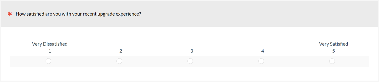
When UX researchers want to measure attitudes and intentions, they often ask respondents to complete multipoint items like the one shown in Figure 1. It’s also common to set a target benchmark for these types of items (e.g., at least 4 on a five-point scale).
This leads to an important question in research planning. How large must the sample size be when comparing the mean of a novel rating scale to a specified benchmark?
All sample size calculations require an estimate of the variability of the metric, expressed as a standard deviation. This is easy for binary data because the standard deviation can be generated from the proportion. For example, if setting a benchmark of 30% top-box scores for a survey item, the sample size can be easily computed because the standard deviation is part of the benchmark (the square root of .3 × .7; see Chapter 6 of Quantifying the User Experience). For more continuous data, you need some idea of the standard deviation (e.g., from analysis of known distributions, a fraction of the maximum range of a scale, or historical data). Of these various methods, historical data is the most accurate. For novel items, however, there is no historical data. So how do you compute the sample size?
In previous articles, we’ve covered how to estimate sample sizes for benchmark testing with the Net Promoter Score (NPS) and the System Usability Scale (SUS). These metrics are well-known, though—far from novel.
Fortunately, we have analyzed our historical standard deviations from a large dataset of 100,000 individual rating scale responses and numerous standardized UX questionnaires.
In this article, we use the analysis of those historical standard deviations to guide sample size estimation for comparisons with benchmark values when the primary outcome measure is the mean of an individual rating scale (e.g., five- or seven-point item) or a multi-item questionnaire.
What Drives Sample Size Requirements for Comparing Rating Scale Means to Benchmarks?
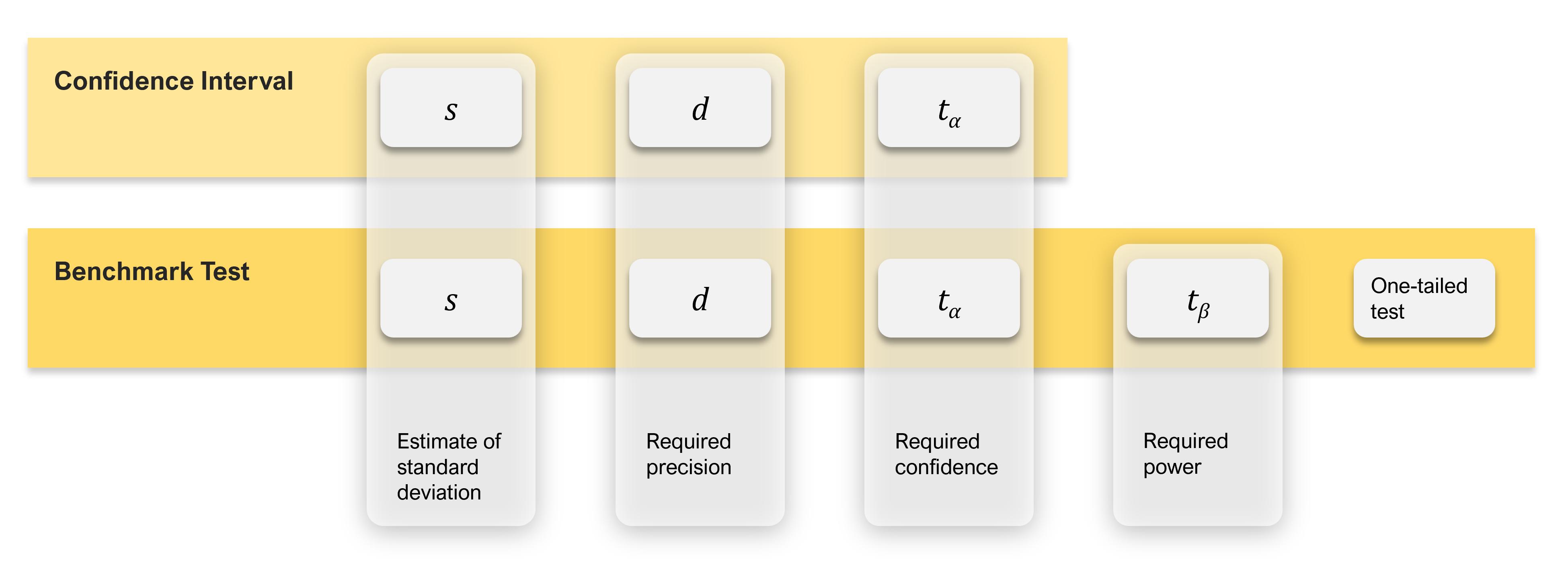
As mentioned, to compute a sample size, at a minimum, you need an estimate of the variability of the measure (standard deviation), but you also need a judgment of the required precision of measurement and a judgment of the desired confidence level. In fact, this is all you need to compute the sample size requirement for studies in which you only plan to compute a confidence interval around a mean.
But when computing the sample size for comparing a mean to a benchmark, you need to know five things. The first three are the same elements required to compute the sample size for a confidence interval.
- An estimate of the rating scale standard deviation: s
- The required level of precision (using points or percentages): d
- The level of confidence (typically 90% or 95%): ta
Sample size estimation for comparing a mean against a set benchmark requires two additional considerations:
- The power of the test (typically 80%): tβ
- The distribution of the rejection region (one-tailed for benchmark tests)
Figure 2 illustrates how the number of sample size drivers increases and changes from confidence intervals (the simplest with three drivers) to benchmark testing (five drivers).
Quick Recap of Power and Tails (Rejection Regions)
The power of a test refers to its capability to detect a specified minimum difference between means (i.e., to control the likelihood of a Type II error). The number of tails refers to the distribution of the rejection region for the statistical test. In the vast majority of cases, comparisons of two rating scale means should use a two-tailed test. However, when comparing a mean to a benchmark, we use a one-tailed test because we almost always care only that the mean beats a certain threshold (e.g., above 4 on a positive-tone five-point item, below 2 on a negative-tone five-point item). For more details on these topics, see the previous article on SUS benchmark testing.
Quick Recap of Typical, Low, and High Standard Deviations for Multipoint Rating Scales and Multi-Item Questionnaires
From our analyses of historical standard deviations and other approaches to estimating unknown standard deviations, we found that a good estimate of the typical (50th percentile) standard deviation of an individual rating scale is about 25% of the maximum range of the scale (e.g., 1 point on a five-point scale). A more conservative estimate (75th percentile) is about 28% of the maximum range of the scale (e.g., 1.12 points on a five-point scale). A good estimate (50th percentile) of the typical standard deviation for a multi-item questionnaire is about 20% of the maximum range of the scale (e.g., 20 points on a 0–100-point scale), which coincidentally is a reasonable estimate of a liberal (25th percentile) standard deviation for individual rating scales (e.g., .8 point on a five-point scale).
Sample Size Formula and Tables for Comparing Means with Benchmarks
To test whether you beat a specified benchmark, you can compare a single mean of scores with a set value (e.g., seeing whether the mean of a five-point scale is greater than 4).
Note that the simple sample size formula in this article works reasonably well when the sample size (n) is greater than 20 but underestimates the requirements when n is smaller. To get the most precise estimate we can, the entries in this article’s tables have been computed using the iterative method described in Quantifying the User Experience.
Also, we expect these sample size estimates for rating scales to be very accurate when item means are close to the midpoint and reasonably accurate until means get close to an endpoint. Because the standard deviations for binary metrics and rating scales approach 0 as means approach a scale endpoint, the actual sample size requirements for extreme means will be smaller than those in the tables. This isn’t a problem when the cost of additional samples is small, but when that cost is high, consider running a pilot study to get an estimate of the actual standard deviation rather than using the tables.
Standardizing Ratings to a 0–100-Point Scale
To standardize the tables in this article so they will work for any number of points in a multipoint scale or multi-item questionnaire, we interpolated the values in the Effect Size columns to a 0–100-point scale. Table 1 shows how these effect sizes (unstandardized mean differences) correspond to equivalent mean differences on five-, seven-, and eleven-point scales. For example, a mean difference of 20 points on a 0–100-point scale is equivalent to a difference of 0.8 on a five-point scale (endpoints from 1 to 5), 1.2 on a seven-point scale (endpoints from 1 to 7), or 2.0 on an eleven-point scale (endpoints from 0 to 10).
| 0–100-pt Scale | 5-pt Scale | 7-pt Scale | 11-pt Scale |
|---|---|---|---|
| 50 | 2.00 | 3.00 | 5.00 |
| 40 | 1.60 | 2.40 | 4.00 |
| 30 | 1.20 | 1.80 | 3.00 |
| 20 | 0.80 | 1.20 | 2.00 |
| 15 | 0.60 | 0.90 | 1.50 |
| 12 | 0.48 | 0.72 | 1.20 |
| 10 | 0.40 | 0.60 | 1.00 |
| 9 | 0.36 | 0.54 | 0.90 |
| 8 | 0.32 | 0.48 | 0.80 |
| 7 | 0.28 | 0.42 | 0.70 |
| 6 | 0.24 | 0.36 | 0.60 |
| 5 | 0.20 | 0.30 | 0.50 |
| 4 | 0.16 | 0.24 | 0.40 |
| 3 | 0.12 | 0.18 | 0.30 |
| 2 | 0.08 | 0.12 | 0.20 |
| 1 | 0.04 | 0.06 | 0.10 |
Table 1: Equivalent effect sizes (mean differences) for 0–100-point scales with five-, seven-, and eleven-point scales.
Comparing a Rating Scale Mean with a Specified Benchmark
The basic sample size formula for a test against a specified benchmark is essentially the same as the one used for confidence intervals, but there are some differences in the details:

Here, s is the standard deviation, t is the summed t-value for the desired level of confidence (ta) AND power (tβ) to control probabilities for Type I (alpha) and Type II (beta) errors, and d is the target for the effect size (the smallest difference that you need to be able to detect between the mean and the benchmark, also known as the critical difference).
For details on setting the values for ta and tβ in this experimental design, see the article “Sample Sizes for Comparing SUS to a Benchmark.” In summary, because a test against a set benchmark is one-sided (i.e., the result is only meaningful when you significantly beat the benchmark), the appropriate value of ta in the formula should be one-sided (e.g., when n > 20, set ta to 1.645 for 95% confidence or 1.282 for 90% confidence). For 80% power (and n > 20), the value of tb is 0.842.
Table 2 shows the sample size estimates for tests against a set benchmark for various effect sizes (minimally detectable differences between the mean and the benchmark, percentage points for binary metrics, scale points for rating scales), four magnitudes of standard deviations (s = 50%, used for binary variables; s = 20, suitable for multi-item questionnaires; s = 25, suitable for individual multipoint rating items; s = 28, suitable for individual multipoint rating items that are suspected to be more variable than the typical item), 95% confidence (i.e., setting the Type I error to .05), and 80% confidence (i.e., setting the Type II error to .20). The only difference in Table 3 is that confidence is 90% (i.e., Type I error set to .10), a common criterion for industrial research.
| Effect Size | Binary Metric, s = 50% | 0–100-Point Rating Scale, s = 20 | 0–100-Point Rating Scale, s = 25 | 0–100-Point Rating Scale, s = 28 |
|---|---|---|---|---|
| 50(%) | 3 | 2 | 2 | 3 |
| 40(%) | 8 | 2 | 4 | 5 |
| 30(%) | 15 | 5 | 6 | 7 |
| 20(%) | 37 | 8 | 12 | 14 |
| 15(%) | 67 | 13 | 19 | 24 |
| 12(%) | 106 | 19 | 29 | 36 |
| 10(%) | 153 | 27 | 41 | 50 |
| 9(%) | 189 | 33 | 50 | 62 |
| 8(%) | 240 | 41 | 62 | 78 |
| 7(%) | 314 | 52 | 81 | 101 |
| 6(%) | 428 | 71 | 109 | 137 |
| 5(%) | 617 | 101 | 157 | 196 |
| 4(%) | 964 | 157 | 244 | 305 |
| 3(%) | 1716 | 277 | 431 | 541 |
| 2(%) | 3863 | 620 | 968 | 1214 |
| 1(%) | 15455 | 2475 | 3866 | 4849 |
Table 2: Sample size estimates for benchmark tests with 95% confidence and 80% power.
| Effect Size | Binary Metric, s = 50% | 0–100-Point Rating Scale, s = 20 | 0–100-Point Rating Scale, s = 25 | 0–100-Point Rating Scale, s = 28 |
|---|---|---|---|---|
| 50(%) | 2 | 2 | 2 | 2 |
| 40(%) | 6 | 2 | 3 | 3 |
| 30(%) | 11 | 4 | 5 | 5 |
| 20(%) | 27 | 6 | 9 | 10 |
| 15(%) | 49 | 10 | 14 | 17 |
| 12(%) | 77 | 14 | 21 | 26 |
| 10(%) | 112 | 20 | 30 | 37 |
| 9(%) | 138 | 24 | 36 | 45 |
| 8(%) | 175 | 30 | 46 | 57 |
| 7(%) | 229 | 38 | 59 | 74 |
| 6(%) | 312 | 52 | 80 | 100 |
| 5(%) | 450 | 74 | 114 | 143 |
| 4(%) | 703 | 114 | 178 | 223 |
| 3(%) | 1251 | 202 | 315 | 394 |
| 2(%) | 2816 | 452 | 706 | 885 |
| 1(%) | 11269 | 1805 | 2819 | 3536 |
Table 3: Sample size estimates for benchmark tests with 90% confidence and 80% power.
For example, to detect a difference of 20 points between a mean and a benchmark with 95% confidence, start in the Effect Size column in Table 2 and move down to the row starting 20(%). The column labeled “Binary Metric, s = 50%” is the sample size needed for a binary metric with that margin of error which, assuming maximum variance, would be 37. Using the typical standard deviation estimate for rating scales (25% of the range) would reduce the sample size to 12. At this level of precision, the sample size for rating scales saves the expense of 25 participants and is about 1/3 the sample size for binary metrics!
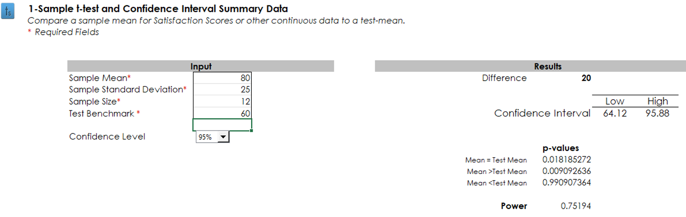
Continuing this example, suppose you’ve set a benchmark to 60 points on a 0–100-point scale, and after you’ve collected data from 12 participants, the mean from the sample is 80 with a standard deviation of 25. The p-value from a t-test should be lower than .05 because the observed mean is exactly 20 points greater than the benchmark with a sample size for 95% confidence and 80% power. As shown in Figure 3, the observed mean is significantly greater than the benchmark (t(11) = 2.77, p = .018), so this result is evidence of having significantly exceeded the benchmark. Note, however, that if the observed mean had been 70—just 10 points higher than the benchmark—the result would not have been significant (t(11) = 1.38, p = .19). Keeping everything else the same, to achieve significance with a 10-point difference would require a sample size of 41.
The savings for rating scales relative to binary metrics is even greater for smaller margins of error. For example, at a margin of error of ±2 points with 95% confidence, you’d need 3,863 participants using a binary metric, but just a quarter of that (968) using the typical rating scale’s standard deviation of 25% of the maximum range (saving the cost of 2,895 participants).
A Few More Examples
Single eleven-point item. Suppose you’ve created a new eleven-point (0–10) item to measure the likelihood that a customer will defect (stop using your product and start using a competitor). The higher the rating, the more likely the customer will defect. You want to test if the mean of a sample of your current customers will be significantly higher than the midpoint of 5, and you want a sample size large enough to detect this as significant when the difference is as small as 1 point on the eleven-point scale. Because the cost of each sample is fairly low, you decide to use the 75th percentile standard deviation from our historical data (28% of the range of the scale) and test with 95% confidence and 80% power.
Start with Table 1 to see what effect size to use in Table 2. A difference of 1 on an eleven-point scale corresponds to a difference of 10 on a 0–100-point scale. The entry in Table 2 (95% confidence) for s = 28 and an effect size of 10 indicates the sample size (n) should be 50. In summary:
- Type of scale: eleven-point item
- Confidence: 95%
- Power: 80%
- Standard deviation: 28%
- Effect size: 1 point on an eleven-point scale (10 points on a 0-100-point scale)
- Sample size: 50
Single five-point item. For a new five-point (1–5) item that measures the clarity of product filter designs on a commercial website, assume you want to know the sample size requirement with a typical standard deviation (25% of the range of the scale) and 90% confidence, 80% power, and an effect size of 1/5 of a point (.20) on the five-point scale.
Start with Table 1 to see what effect size to use in Table 3 (90% confidence). For a five-point scale, a difference of .20 corresponds to 5 points on a 0–100-point scale. The sample size in Table 3 for s = 25 and an effect size of 5 is n = 114. In summary:
- Type of scale: five-point item
- Confidence: 90%
- Power: 80%
- Standard deviation: 25%
- Effect size: .20 points on a five-point scale (5 points on a 0–100-point scale)
- Sample size: 114
Multi-item questionnaire. You have three new seven-point items that measure different aspects of website attractiveness, and you plan to report scores for this questionnaire based on averaging the three ratings and then interpolating the values to a 0–100-point scale. You set the benchmark for an adequate level of attractiveness at 70 and want to know the sample size requirement for 90% confidence and 80% power using the typical standard deviation for multi-item questionnaires (20% of the scale range), which will indicate statistical significance when the mean is at least 7 points higher than the benchmark.
Because the scale in this example ranges from 0 to 100, you can start directly in Table 3 (90% confidence). The sample size for an effect size of 7 when s = 20 is n = 38. In summary:
- Type of scale: Multi-item questionnaire
- Confidence: 90%
- Power: 80%
- Standard deviation: 20%
- Effect size: 7 points on a 0–100-point scale
- Sample size: 38
Summary and Takeaways
What sample size do you need when comparing rating scale means with set benchmarks? To answer that question, you need several types of information, some common to all sample size estimation (confidence level to establish control of Type I errors, standard deviation, and margin of error or critical difference), others unique to statistical hypothesis testing (one- vs. two-tailed testing, setting a level of power to control Type II errors).
The “right” sample size depends on the research details. If accurate estimates of binary metrics are a critical part of your research, use the sample sizes in the binary metrics column in the tables because those sample sizes will also be more than adequate for your rating scale analyses. If your primary analyses will be rating scales, in most cases, you can use the “s = 25” column (but if you have concerns that your standard deviations might be larger than average, use the “s = 28” column). If your primary analyses will be multi-item questionnaires, you can reasonably use the “s = 20” column.
Balance statistics and logistics. When planning a study, these tables help researchers balance statistics and logistics. The math for significantly detecting a difference of one point between a rating scale mean and a benchmark may indicate aiming for a sample size over 1,500, but the cost and time of obtaining that many participants might be prohibitive, even in a retrospective survey or unmoderated usability study where the cost of each sample is fairly low.
Using rating scale standard deviations instead of binary significantly reduces sample sizes. If your primary measure in a survey or benchmark study is a rating scale, using sample size calculations for rating scales instead of using binary data at maximum variance provides significant savings. Typical sample size requirements for binary metrics are two to four times as large as those required for rating scales. At its maximum value (p = .5), the standard deviation of binary metrics is 50% of the range of the binary scale (from 0 to 100%). For individual multipoint items, our estimate of typical standard deviations is about 25% of the maximum scale range.
Look for the Goldilocks zones. We borrow the term Goldilocks zone from astronomy, where it refers to planets that are just the right distance from their suns to have liquid water. In each of the tables in this article, there are a group of sample sizes that are “just right” for their balance between sensitivity and attainability. For many research studies, sample sizes as high as 500 are affordable, and effect sizes as low as 10 are sufficiently sensitive. For example, for rating scales with s = 25 in Table 2, the Goldilocks zone ranges from effect sizes of 10 to 3 with corresponding sample sizes from 41 to 431. You can adjust these sensitivity and attainability goals as needed for your research context.