 The UX-Lite® is a relatively new but increasingly popular metric for UX research.
Its two items generate an overall score and subscale scores on ease and usefulness from 0 to 100. The UX-Lite predicts future product usage as well as or better than the original and longer Technology Acceptance Model (TAM). The ease score also predicts the SUS with over 95% accuracy.
One of the benefits of the UX-Lite is its familiar scoring system from 0 to 100 (like the SUS) and its reasonable set of benchmark scores.
Finding the right sample size estimate isn’t about picking a magic number. While there may be some magic ranges, the right process involves starting with the type of study design.
Three of the most common UX study designs are those with a focus on estimation with confidence intervals (discussed in a previous article), comparison with a benchmark, and comparison of two means.
Across all three study types, a key ingredient is the historical standard deviation of the UX-Lite. Fortunately, we’ve collected enough data to have a good idea about a typical UX-Lite standard deviation.
In this article, we demonstrate how to compute the right sample size for comparing UX-Lite scores to a benchmark by controlling the size of the critical difference (i.e., the desired level of precision, specifically, the smallest difference you need to be able to reliably detect).
What Drives Sample Size Requirements for Benchmark Tests?
Not to be intentionally confusing, but we often use “benchmark testing” to mean a few things. First, it’s used loosely to refer to the process of collecting metrics (e.g., benchmarking), which we cover extensively in Benchmarking the User Experience.
It also refers to how metrics collected within a study will be used. They can be used to establish the current experience of a product (a new benchmark), in which case you would use confidence intervals around the benchmark to assess its precision.
Metrics can also be used to compare against a prior experience or a competitive experience (comparative or competitive) or to compare against established thresholds (a benchmark). We’re focusing on this final case, where a sample of UX-Lite scores is collected, and then the mean UX-Lite score is compared to a set benchmark value.
As shown in Figure 1, you need to know five things to compute the sample size for a comparison to a benchmark. The first three are the same elements required to compute the sample size for a confidence interval (for a comprehensive discussion of these three elements, see our previous article).
- An estimate of the UX-Lite standard deviation (median of 19.3 with an interquartile range from 16.6 [25th percentile] to 21.3 [75th percentile]): s
- The level of confidence (typically 90% or 95%): t
- The desired precision of measurement (critical difference): d
Sample size estimation for benchmark tests also requires two additional considerations:
- The power of the test
- The level of confidence for a one-sided (one-tailed) test
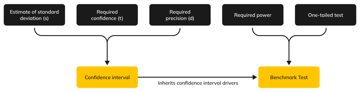
Figure 1: Drivers of sample size estimation for benchmark comparisons.
Power
The power of a test refers to its capability to detect a difference between observed measurements and hypothesized values when there really is a significant difference. The power of a test is not an issue when you’re just estimating the value of a parameter, but it matters when testing a hypothesis. Analogous to setting the confidence level to 1 − α (the acceptable level for Type I errors, or false positives), power is 1 − β (the acceptable level for Type II errors, or false negatives).
One-Tailed Testing
Most statistical comparisons use a strategy known as two-tailed testing. The term “two-tailed” refers to the tails of the distribution of the differences between the two values. The left distribution in Figure 2 illustrates a two-tailed test showing the rejection criterion (α = .05) evenly split between the two tails.
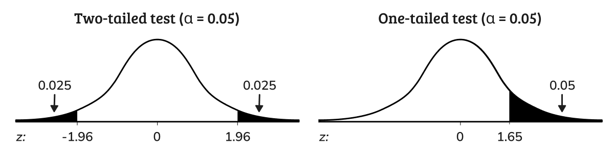
Figure 2: Two- and one-sided rejection regions for two- and one-sided significance tests.
For most comparisons, two-tailed tests are appropriate. When you test an estimated value against a benchmark, however, you care only that your estimate is significantly better than the benchmark. When that’s the case, you can conduct a one-tailed test, illustrated by the right distribution in Figure 2. Instead of splitting the rejection region between two tails, it’s all in one tail. The practical consequence is that the bar for declaring significance is lower for a one-tailed test.
The area in one tail for a two-sided test with α = .10 is the same as a one-sided test with α = .05. This factor decreases the sample size relative to computing a two-tailed confidence interval.
Putting the Values Together
With the five ingredients ready, we use the following formula:
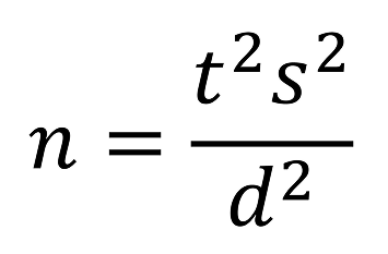
where s is the standard deviation (s2 is the variance), t is the t-value for the desired level of confidence AND power, and d is the targeted size for the interval’s margin of error (i.e., precision).
A difference compared to the confidence interval computation is that t is actually the sum of two t-values, one for α (related to confidence) and one for β (related to power, always one-sided). For a 90% confidence level and 80% power, this works out to be about 1.645 + 0.842 = 2.5.
When you don’t need more power, the default power level is 50%, at which t for power = 0, making it the same result as a confidence interval. Any larger value for power (commonly 80%) makes the value of t larger, which will increase the estimated sample size.
One way to think of including power in sample size estimation is as an insurance policy that you purchase by increasing your sample size to increase your likelihood of finding statistically significant results if the standard deviation is a little higher than expected or the observed value of d is a bit lower.
Sample Size Table for UX-Lite Benchmark Comparisons
Table 1 shows how variations in these three components affect sample size estimates for confidence intervals for the median standard deviation of 19.3 and for the 75th percentile of 21.3. In most cases, it’s reasonable to use the median standard deviation, but when a sufficient sample size is more important than the cost of sampling, it’s better to plan with the higher value.
| d | |||||
| 15 | |||||
| 10 | |||||
| 7.5 | |||||
| 5.0 | |||||
| 2.5 | |||||
| 2.0 | |||||
| 1.0 | |||||
Table 1: Sample size requirements for UX-Lite benchmark comparisons given various standard deviations (s), confidence levels, and critical differences (d), with power set to 80% (green shading shows the “magic range” for this table).
For example, to declare that you have significantly beaten a UX-Lite benchmark of 75 with 90% confidence, 80% power, a standard deviation of 19.3, and a critical difference of 15, you will need a sample size of 9, but you will also need the observed UX-Lite mean to be 90 (75 + 15) or higher.
At the other end of the table, if you have the same benchmark (75), 95% confidence, 80% power, a standard deviation of 21.3, and a critical difference of 1, you’ll only need the observed UX-Lite mean to be 76 (75 + 1), but you’ll need a sample size of 2,807.
In this table, the “magic range” for the critical difference is from 2.5 to 5, where the sample sizes are reasonably attainable (n from 69 to 451). The table also illustrates the tradeoff between the ability of a test to detect significant differences and the sample size needed to achieve that goal.
Technical Note: What to Do for Different Standard Deviations
If your historical UX-Lite data has a very different standard deviation from 19.3 or 21.3, you can do a quick computation to adjust the values in these tables. The first step is to compute a multiplier by dividing the new target variance (the square of the standard deviation, s2) by the variance used to create the table. Then multiply the tabled value of n by the multiplier and round it to get the revised estimate. To illustrate this, we’ll start with a standard deviation of 19.3 (our typical standard deviation) and show how this works if the target standard deviation (s) is 21.3 (our conservative estimate in Table 1). The target variability (21.32) is 453.69. The initial variability is 372.49 (19.32), making the multiplier 453.69/372.49 = 1.218. To use this multiplier to adjust the sample size for 95% confidence and precision of ±2.5 shown in Table 1 when s = 19.3, multiply 370 by 1.218 to get 450.66 then round it to 451. For more information, see our article, How Do Changes in Standard Deviation Affect Sample Size Estimation.
Summary and Takeaways
What sample size do you need when conducting a UX-Lite benchmark test? To answer that question, you need several types of information, some common to all sample size estimation (confidence level to establish control of Type I errors, standard deviation, margin of error or critical difference) and others unique to statistical hypothesis testing (one- vs. two-tailed testing, setting a level of power to control Type II errors).
We provided a sample size table based on a typical standard deviation for the UX-Lite in retrospective UX studies (s = 19.3) and a more conservative standard deviation (s = 21.3), with examples of its use.
For UX researchers working in contexts where the typical standard deviation of the UX-Lite might differ, we provided a simple way to increase or decrease the tabled sample sizes for larger or smaller standard deviations. While there isn’t a magic number that will always work, in practice, there are ranges that satisfy many requirements. When comparing UX-Lite scores to benchmarks given measurement precision from 2.5 to 5 points and the typical standard deviation of 19.3, the sample sizes range from 69 to 370.


